Axiomatic Approach to Probability: Probability is the certainty that an event will occur. It is a field of Mathematics dealing with numerical explanations of the chance of an event occurring or the truth of a statement. Probability can only be applied to experiments in which the complete number of outcomes is known, i.e., the idea of probability cannot be applied unless the total number of outcomes of an experiment is known.

Hence, we need to know the total number of possible outcomes of the experiment to apply probability in everyday situations. Axiomatic probability is an approach to expressing the probability of an event occurring. Several axioms or rules are predefined before assigning probabilities. This is done to quantify the event and make calculating the occurrence or non-occurrence of events easier.

Axiomatic Approach to Probability: Overview

One of the techniques to describe the probability of an event occurring is to use an axiomatic approach. We are familiar with random experiments, sample space, and occurrences related to probability experiments. We use various terms regarding the probability of events occurring in our daily lives, such as weather forecasts, buying and selling. Probability theory measures the probability of events occurring or not occurring.

The theoretical probability of an event is the ratio of the number of outcomes to the total number of outcomes. In contrast, the axiomatic approach is quite different. In this approach, some axioms or rules are depicted to assign probabilities.

Axiomatic probability is a theory that unifies probability. It establishes a set of axioms (laws) that apply to all types of probability, including frequentist and classical probabilities. Based on Kolmogorov’s three axioms, these laws establish the starting points of mathematical probability.

Classical and Axiomatic Approach

This method is based on the assumption that all outcomes are equally likely. Suppose an event can occur in \(n\) different ways out of a total of \(N\) possibilities. The earliest probability is the classical probability, typically applied to simple scenarios such as a gambling game. Assume a random experiment (such as a roll of the dice) yields a finite number, \(n\) of equally likely possibilities. If  \(m\) of the outcomes have a unique feature, the probability of that characteristic is the ratio \(\frac{m}{n}\). This is effective for examining dice throws and card picks, but it is less useful in complex scenarios.

Frequentist Probability

This method of estimating probability is more general. It does not assume that all of the possible outcomes are equally likely. We repeat the experiment numerous, let’s say \(M\) times, when the results are not equally likely. Then, count how many times that same output occurred, say \(m\). Lastly, come up with an empirical probability estimate. Hence, we use of the relationship shown below.
\(P\left( {{\text{event}}} \right) = {\log _{M \to \infty }}\frac{m}{M}\)

The value of empirical probability should only be used when the experiment is performed infinite times.

Finally, both approaches fail to withstand the rigours of Mathematics because the former incorporates the uncertain phrase, “equally likely,” for which there is no mathematical justification. The latter lacks a way to prove that \({\log _{M \to \infty }}\frac{m}{M}\)  will cover some value because no experiment can be repeated infinite times.

Axioms

The axiomatic approach to probability considers probability as a function associated with any event, even if the event is unlikely.

Axiom 1

Statement: The probability of every given event \(X\) must be greater than or equal to zero. Thus,
\(0 \leqslant P\left( X \right)\)
The probability of an event defined on the sample space is larger than or equal to zero, according to Axiom \(1\). If the sample space has \(n\) points, the impossible event, that is, an event with no sample points, is the empty event on \(S\) with a probability of zero. This event is denoted by \(\emptyset \).
\(P\left( \emptyset  \right) = \frac{0}{n}\)
\(\therefore \,P\left( \emptyset  \right) = \,0\)

Axiom 2

Statement: The set of all the outcomes is known to be the sample space \(S\) of the experiment. This suggests that the chance of every given outcome occurring is \(100\% \) or \(P\left( S \right) = 1\). Intuitively, this suggests a \(100\% \) chance of achieving a specific result whenever this experiment is performed.
\(P\left( S \right) = 1\)
The probability of \(S\), the sample space, is one, according to Axiom \(2\). That is to say,
\(P\left( S \right) = \frac{n}{n}\)
\(\therefore P\left( S \right) = 1\)

 Note that if we calculate the likelihood of each event on the sample space \(S\), we call it a probability space.

Furthermore, if we add up the probabilities of all possible simple events on \(S\), we get one or \(100\% \). 

Axiom 3

Statement: For the experiments with two outcomes,  \(A\) and \(B\), if \(A\) and \(B\) are mutually exclusive, then
\(P\left( {A \cup B} \right) = P\left( A \right) + P\left( B \right)\)
The probability of the union of more than one event on \(S\) equals the total of their probabilities, according to Axiom \(3\), assuming that the sequence of events is mutually exclusive. You may recall that if \({A_{1\,}} \cap \,\,{A_2} = \emptyset \), two occurrences \({A_{1\,}}\) and \({A_{2\,}}\) in \(S\) are said to be mutually exclusive. Every feasible pair in the sequence must be mutually exclusive to satisfy the condition.

Conditions of Axiomatic Approach

For the events \({A_1},\,{A_2},\,……{A_n}\) defined in the sample space \(S\). The probability of each event, denoted by \(P\left( {{A_i}} \right)\) where \(i = 1,\,2,….n,\) are numbers that satisfy the following three conditions:
1. \(0 \leqslant P\left( {{A_i}} \right)\)
2. \(P\left( S \right) = 1\,{\text{or }}P\left( {{A_1}} \right) + P\left( {{A_2}} \right) \pm …… + P\left( {{A_n}} \right) = 1\)
3. \(P\left( {{A_1}\, \cup \,{A_2}\, \cup ……{A_n}} \right) = P\left( {{A_1}} \right) + P\left( {{A_2}} \right) + ….P\left( {{A_n}} \right)\) where \({A_1},\,{A_2},\,……{A_n}\) are mutually exclusive events.

Probability of Equally Likely Outcomes

Equally likely events are those that have the same theoretical probability (or likelihood) of occurrence.

Example: When a die is tossed, each number getting on a die is equally likely to occur. The probability of getting each number on a die is \(\frac{1}{2}\).

Probability of OR Events

The probability of ‘\(A\) or \(B\)’ is calculated as \(P\left( {A\,{\text{or}}\,B} \right) = P\left( A \right) + P\left( B \right)\), where \(A\) and \(B\) are mutually exclusive events.

Example: The events of getting even numbers or odd numbers are mutually exclusive. The probability of such events is \(P\left( {{\text{Even}}\,{\text{or}}\,{\text{Odd}}} \right) = \frac{1}{2} + \frac{1}{2} = 1\).

Probability of Complementary Events

Two events are complementary events when one event occurs if and only if the other does not. The sum of probabilities of two complementary events is one.

Example: Getting a head or a tail is a complementary event.

\(P\left( {{\text{head}}} \right) = 1 – P\left( {{\text{tail}}} \right) = \frac{1}{2}\)

Applications of Axiomatic Approach

• Probability theory is used in risk assessment and modelling in everyday life. Actuarial science is used by the insurance sector and markets to calculate prices and make choices.
• Probability can also be used to examine trends in biology (for example, disease spread) and ecology.
• Probability and ancient game references, market surveys, and player inputs are used to build games.
• In natural language processing, the cache language model and other statistical language models are instances of probability theory applications.

Summary

The classical probability of an event is finding the possibility of equally likely outcomes, and it is the ratio of favourable outcomes to the total outcomes.

For checking the non-equally likely outcomes, Andrey Kolmogorov developed Kolmogorov laws in 1933. The axiomatic approach is finding the probability by applying some rules or axioms.

The three laws of Kolmogorov are the law of impossible, sum of elementary events and mutually exclusive events. They tell the probability of an impossible event and sure event, the sum of probabilities of event and also that of mutually exclusive events.

The probability of equally lightly outcomes is same for each outcome. probability of mutually exclusive events is the sum of probabilities of the events.

Solved Examples

 Q1. If an unbiased coin was tossed three times, what is the probability of getting three heads or three tails?
Solution:
The number of events in a sample space of tossing a coin three times is given by the formula \({2^n}\), where \(n\)is the number of coins tossed.
So, total outcomes in a sample space, \({2^3} = 2 \times 2 \times 2 = 8\)
\(S = \left\{ {HHH,\,HHT,HTH,HTT,THH,THT,TTH,TTT} \right\}\)
The events getting three heads \(\left( A \right) = \left\{ {HHH} \right\}\)
The events getting three tails \(\left( B \right) = \left\{ {TTT} \right\}\)
Here, the event of getting three heads and three tails are mutually exclusive events.
So, probability \( = \frac{{{\text{favorable}}\,{\text{outcomes}}}}{{{\text{total}}\,{\text{number}}\,{\text{of}}\,{\text{outcomes}}}}\)
Probability of getting all three as heads or tails is given by
\(P\left( {A\,{\text{or}}\,B} \right) = P\left( A \right) + P\left( B \right) = \frac{1}{8} + \frac{1}{8} = \frac{2}{8} = \frac{1}{4}\)

Q2. If \(\frac{2}{{11}}\) is the probability of an event, what is the probability of the event “not \(A\)”?
Solution:
Probability \( = \frac{2}{{11}}\)
Sum of probabilities of two complementary events is one.
Probability of \(A\) is the complementary event \((A’)\) of the given event.
\(P\left( A \right) + P\left( {A’} \right) = 1\)
\(P\left( {A’} \right) = 1 – \frac{2}{{11}}\)
\( = \frac{{\left( {11 – 2} \right)}}{{11}}\)
\(\therefore \,P\left( {A’} \right) = \frac{9}{{11}}\)
Hence, the probability of the event \(A’\) is \(\frac{9}{{11}}\).

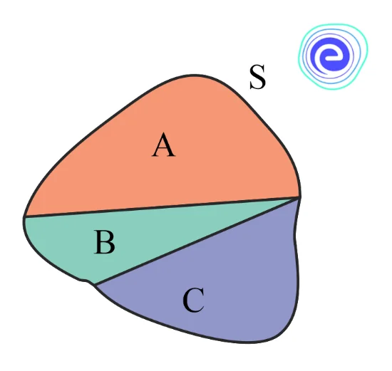
Q3. If an experiment has exactly the three possible mutually exclusive outcomes \(A, B\) and \(C\) check each case whether the assignment of probability is permissible
\(P\left( A \right) = \frac{4}{7},P\left( B \right) = \frac{1}{7},\,P\left( C \right) = \frac{2}{7}\)
Solution:
Since the experiment has three possible mutually exclusive outcomes \(A, B\) and \(C\), they are exhaustive events.
\( \Rightarrow S = A \cup B \cup C\)

Therefore, using the axioms of probability, we get
\(P\left( A \right) \geqslant 0,P\left( B \right) \geqslant 0,P\left( C \right) \geqslant 0\,{\text{and}}\,P\left( {A \cup B \cup C} \right) = P\left( A \right) + P\left( B \right)9 + P\left( C \right)\)
\( = P\left( S \right) = 1\)
\( \Rightarrow \frac{4}{7} + \frac{1}{7} + \frac{2}{7} = \frac{{4 + 1 + 2}}{7} = \frac{7}{7} = 1\)
So, the given probabilities are permissible.

Q4. Find out the probability of getting a number less than \(7\) when a die is tossed. 
Solution:
We know that possible outcomes when a die is tossed are \(\left\{ {1,\,2,\,3,\,4,\,5,\,6} \right\}\)
The numbers less than \(7\) are \(1, 2, 3, 4, 5, 6\)
Number of favourable outcomes \(=6\)
Total number of outcomes \(=6\)
So, the probability of getting a number less than \(7\) is given by
\(P\left( {n < 7} \right) = \frac{6}{6}\)
\(\therefore \,P\left( {n < 7} \right) = 1\)

Q5. A bag has \(5\) red balls and \(3\) black balls. Find out the probability of getting a ball and verify the second axiom.
Solution:
Let us define two events,
\(R=\) Red ball is picked 
\(B=\) Black Ball is picked
Probability of getting a red ball is \(P\left( R \right) = \frac{5}{8}\)
Probability of getting a black ball is \(P\left( B \right) = \frac{3}{8}\)
\(P\left( R \right) + P\left( B \right) = \frac{5}{8} + \frac{3}{8}\)
\( = \frac{8}{8}\)
\(\therefore P\left( R \right) + P\left( B \right) = \,1\,\)
Thus, the second axiom is also satisfied.

Frequently Asked Questions (FAQs)

Q1. What are the 3 axioms of probability?
Ans: For the events \({A_1},\,{A_2},\,……{A_n}\) be events defined on the sample space S. The three axioms of probability is given by
1. \(0 \leqslant P\left( {{A_i}} \right)\)
2. \(P\left( S \right) = 1\)
3. \(P\left( {{A_1}\, \cup \,{A_2}\, \cup ……{A_n}} \right) = P\left( {{A_1}} \right) + P\left( {{A_2}} \right) + ….P\left( {{A_n}} \right)\) where \({A_1},\,{A_2},\,……{A_n}\) are mutually exclusive events.

Q2. What are two approaches of probability?
Ans: The two approaches to probabilities are:
1. Classical approach
2. Axiomatic approach

Q3. What is the meaning of the axiomatic approach?
Ans: The axiomatic approach to probability considers probability as a function associated with any event, even if the event is unlikely, which follows certain rules or axioms.

Q4. How do we calculate the classical probability?
Ans: Classical probability of the \(n\) things of total \(m\) things are given by the ratio of \(m\) to \(n\).
\(P\left( {{\text{event}}} \right) = \frac{n}{m}\)

Q5. Who is well known for the axiomatic approach in probability?
Ans: Andrey Kolmogorov developed the Kolmogorov Axioms in 1933, which is the bases of the development of axiomatic approach.