Derivative of a Function: Differentiation in calculus can be applied to measure the function per unit change in the independent variable. We know how to find the slope of a straight line. It is simply the change in \(y\) by the change in \(x\). This is commonly known as the rate of change. While this works well for straight lines, what happens when we find the slope of a nonlinear function? Will the same approach work? The answer is no.

The derivative, which is the instantaneous rate of change or the slope of the tangent at a specific point of a function, can help us overcome this challenge. Let us see how the derivative of a function can be found at a given point by using the concept of limits.

Derivative of a Function

The derivative of a function \(y = f\left( x \right)\) of a variable \(x\) is a measure of the rate at which the value \(y\) of the function changes with respect to the change of the variable \(x\). It is called the derivative of \(f\left( x \right)\) with respect to \(x\).

Let \(f\left( x \right)\) be a function whose domain consists of those values \(x\) of such that the following limit exists.

\(f’\left( x \right) = {\mkern 1mu} \mathop {\lim }\limits_{h \to 0} {\mkern 1mu} \frac{{f\left( {x + h} \right) – f\left( x \right)}}{h}\)

Learn About Relations and Functions Here

As a Measure of Rate

In Mathematics, differentiation can be defined as a derivative of a function with respect to an independent variable.

Let \(f\left( x \right)\) be a function of \(x\) and let \(y = f\left( x \right)\). Here, the value of \(y\) is dependent on the value of \(x\), and it changes with a change of in the value of \(x\). So \(x\) is called the independent variable, and \(y\) is the dependent variable.

Let \(\Delta x\) be a small change in \(x\), and let \(\Delta y\) be the correspondence change in \(y = f\left( x \right)\). Then, the value of \(x\) changes from \(x\) to \(x + \Delta x\), and the value of \(f\left( x \right)\) changes from \(f\left( x \right)\) to \(f\left( {x + \Delta x} \right)\). So, the change in the value of \(f\) is from \(f\left( {x + \Delta x} \right)….\left( i \right)\)

Thus, we observe that due to change \(\Delta x\) in \(x\), so there is a change \(\Delta y\) in \(y\). Therefore, due to unit change in \(x\), change in \(y\) is equal to \(\frac{{\Delta y}}{{\Delta x}}\). This is also known as the average rate of change of \(y\) with respect to the change in \(x\).

As \(\Delta x \to 0\), we observe that \(\Delta y\) also tends to zero.

\(\therefore \) Instantaneous rate of change of \(y\) with respect to \(x = \mathop {\lim }\limits_{\Delta x \to 0 } \frac{{\Delta y}}{{\Delta x}}\)

If we use the phrase rate of change instead of instantaneous rate of change, we have,

Rate of change in \(y\) with respect to change in \(x = \mathop {\lim }\limits_{\Delta x \to 0 } \frac{{\Delta y}}{{\Delta x}}\)

\(= \mathop {\lim }\limits_{\Delta x \to 0} \frac{{f\left( {x + \Delta x} \right) – f\left( x \right)}}{{\Delta x}}\)

\(= \frac{d}{{dx}}\left( {f\left( x \right)} \right)\)

\( = \frac{{dy}}{{dx}}\)

Thus,\( \frac{{dy}}{{dx}}\) or \(\frac{d}{{dx}}\left( {f\left( x \right)} \right)\)  measures the rate of change of \(y = f\left( x \right)\) with respect to \(x\).

\(\therefore \,\frac{{dy}}{{dx}} = \mathop {\lim }\limits_{\Delta x \to 0 } \frac{{\Delta y}}{{\Delta x}}\)

Note:

We know that \( \frac{{dy}}{{dx}}\) or \(\frac{d}{{dx}}\left( {f\left( x \right)} \right)\) is the derivative or differentiation of \(y = f\left( x \right)\). It also measures the rate of change in \(y\) with respect to \(x\). So, we can say that the derivative of \(y = f\left( x \right)\) is the same as the rate of change of \(f\left( x \right)\) with respect to \(x\).

Derivative of a Function at a Point

Let \(f\left( x \right)\) be a real-valued function defined in an open interval \(\left( {a,b} \right)\) and let \(c \in \left( {a,b} \right)\). Then \(f\left( x \right)\) is said to be differentiable at \(x = c\), if \(\mathop {\lim }\limits_{x \to c} \,\frac{{f\left( x \right) – f\left( c \right)}}{{x – c}}\) exists finitely. This limit is called the derivative or differentiation of \(f\left( x \right)\) at \(x = c\), and it is denoted by,

\(f’\left( c \right)\) or \(D\,f\left( c \right)\) or \({\left\{ {\frac{d}{{dx}}f\left( x \right)} \right\}_{x = c}}\)

i.e., \(f’\left( c \right) = \mathop {\lim }\limits_{x \to c} \frac{{f\left( x \right) – f\left( c \right)}}{{x – c}}\), provided that the limit exists.

In this article, it will be assumed that a given function \(f\left( x \right)\) is differentiable at every point of its domain, i.e. \(\mathop {\lim }\limits_{x \to c} \frac{{f\left( x \right) – f\left( c \right)}}{{x – c}}\) exists for all \(c\) in its domain.

Let \(f\left( x \right)\) be a real-valued function differentiable at every point of its domain. Then, corresponding to every point \(c\)in the domain, we obtain a unique real number equal to the derivative of \(f’\left( c \right)\) of \(f\left( x \right)\) at \(x = c\).

Thus, there is a one-to-one correspondence between the points and derivatives at these points. This correspondence induces a function such that the image of any point \(x\) in the domain is the value of derivative of \(f\) at \(x\)

i.e.,\(f’\left( x \right)\) or \(\frac{d}{{dx}}\left( {f\left( x \right)} \right)\) is called the derivative or differentiation of \(f\left( x \right)\) and it is given by

\(f’\left( x \right) = \mathop {\lim }\limits_{h \to 0} \frac{{f\left( {x + h} \right) – f\left( x \right)}}{h}\)

So, finding the derivative of a function using the above formula is the differentiation or derivative from the first principle.

Example: Find the derivative of the function \(f\left( x \right) = \sin \,x\) at \(x=0\).
Solution:
Given that, we have: \(f\left( x \right) = \sin \,x\)
As we know, \(f’\left( c \right) = \mathop {\lim }\limits_{x \to c} \frac{{f\left( x \right) – f\left( c \right)}}{{x – c}}\)
Therefore, \(f’\left( 0 \right) = \mathop {\lim }\limits_{h \to 0} \frac{{f\left( {0 + h} \right) – f\left( 0 \right)}}{h}\)
\(= \mathop {\lim }\limits_{h \to 0} \frac{{\sin \,h – \,\sin \,0}}{h}\)
\( = \mathop {\lim }\limits_{h \to 0} \frac{{\sin \,h}}{h}\)
\( = 1\,\left[ {{\text{Using}}\,\,\mathop {\lim }\limits_{x \to 0} \frac{{\sin \,ax}}{x} = a} \right]\)

Physical Interpretation of Derivative at a Point

Let a particle be moving in straight line from the point \(o\) towards \(x\) as shown in figure.

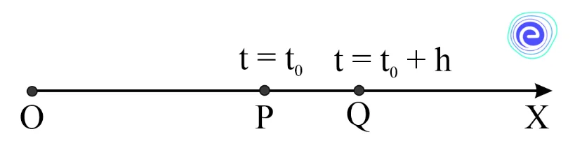
The position of the particle at any time \(t\) depends upon the time elapsed. In other words, the distance of the particle from \(o\) depends upon the time of movement, i.e., it is a function \(f\) of time \(t\) taken by the particle.

Let at any time, say \({t_0}\), the particle be at \(p\), and after further time \(h\) i.e., at \(t = {t_0} + h\) the particle is at \(Q\)

\(\therefore \,OP = f\left( {{t_0}} \right)\) and \(OQ = f\left( {{t_0} + h} \right)\)

Distance travelled in time, \(h = PQ = OQ – OP = f\left( {{t_0} + h} \right) – f{\left( {{t_0}} \right)_{\,\,}}\,\,\,\,\,\,\,\,\)

Average speed of the particle during the journey from the point \(p\) to \(Q = \frac{{PQ}}{h}\)

\(= \frac{{f\left( {{t_0} + h} \right) – f\left( {{t_0}} \right)}}{h}\)

As \(h \to 0\), we observe that \(\,Q \to P\),

\(\therefore \) Instantaneous speed at time \(t = {t_0},\,\mathop {\lim }\limits_{h \to 0} \,\frac{{f\left( {{t_0} + h} \right) – f\left( {{t_0}} \right)}}{h} = f’\left( {{t_0}} \right)\)

Example: The distance, \(f\left( t \right)\) in meters, moved by a particle travelling in a straight line in \(t\) seconds is given by \(f\left( t \right) = {t^2} + 3t + 4\). Find the speed of the particle at the end of \(2\) seconds.
Solution:
Given: \(f\left( t \right) = {t^2} + 3t + 4\)
The speed of the particle at the end of \(2\)seconds is given by \(f’\left( 2 \right)\) which is the derivative of the function at a point \(t = 2\).
Therefore, \(f’\left( 2 \right) = \mathop {\lim }\limits_{h \to 0} \frac{{f\left( {2 + h} \right) – f\left( 2 \right)}}{h}\)
\( \Rightarrow f’\left( 2 \right) = \mathop {\lim }\limits_{h \to 0} \frac{{{{\left( {2 + h} \right)}^2} + 3\left( {2 + h} \right) + 4 – \left\{ {{2^2} + 3 \times 2 + 4} \right\}}}{h}\)
\( \Rightarrow f’\left( 2 \right) = \mathop {\lim }\limits_{h \to 0} \frac{{\left( {{h^2} + 7h + 14} \right) – 14}}{h}\)
\( \Rightarrow f’\left( 2 \right) = \mathop {\lim }\limits_{h \to 0} \frac{{\left( {{h^2} + 7h} \right)}}{h}\)
\( \Rightarrow f’\left( 2 \right) = \mathop {\lim }\limits_{h \to 0} \left( {h + 7} \right)\)
\( \Rightarrow f’\left( 2 \right) = 7\)
Hence, the speed of the particle at the end of \(2\)seconds is \(7\,{\text{m/s}}\)

Geometrical Interpretation of Derivative at a Point

Let \(f\left( x \right)\) be a differentiable function. Consider the curve \(y = f\left( x \right)\). Let \(p\left( {c,f\left( c \right)} \right)\) be a point on the curve \(y = f\left( x \right)\) and \(Q\left( {c + h,f\left( {c + h} \right)} \right)\) be a neighbouring point on the curve.

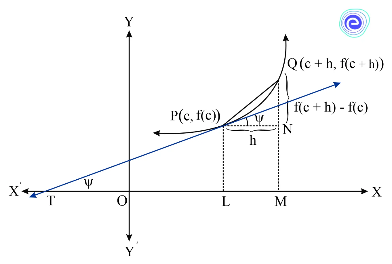
Thus, slope of chord \(PQ = \tan \angle QPN = \frac{{QN}}{{PN}} = \frac{{f\left( {c + h} \right) – f\left( c \right)}}{h}…….\left( i \right)\)

Taking limit as \(Q \to P\) i.e \(h \to 0\) , we obtain \(\mathop {\lim }\limits_{Q \to P} \left( {{\text{Slope}}\,{\text{of}}\,{\text{chord}}\,PQ} \right) = \mathop {\lim }\limits_{h \to 0} \frac{{f\left( {c + h} \right) – f\left( c \right)}}{h}\)

Similarly, as \(Q \to P\), then chord \(PQ\) tends to the tangent to \(y = f\left( x \right)\) at a point \(P\)
Therefore, from equation (i), we get:

Slope of the tangent at \(P = \mathop {\lim }\limits_{h \to 0} \frac{{f\left( {c + h} \right) – f\left( c \right)}}{h}\)

\( \Rightarrow \) Slope of the tangent at \(P = f’\left( c \right)\) i.e., \(\tan \psi  = f’\left( c \right)\), where \(\psi \) is the inclination of the tangent to the curve \(y = f\left( x \right)\) at a point \(\left( {c,f\left( c \right)} \right)\) with respect to the \(x – \)axis.

So, the derivative of the function \(y = f\left( x \right)\) which is \(f’\left( c \right)\), at a point \(x = c\) is the slope of the tangent to the curve \(y = f\left( x \right)\) at the point \(\left( {c,f\left( c \right)} \right)\).

Example: Find the slope of the tangent to the curve \(f\left( x \right) = {x^2}\) at a point \(x =  \,- 2\).
Solution:
Given: \(f\left( x \right) = {x^2}\)
The slope of the tangent to the curve \(f\left( x \right) = {x^2}\) at a point \(x = \, – 2\) is \(f’\left( { – 2} \right)\).
In other words, the derivative of the function \(f\left( x \right)\) at \(x = \, – 2\).
Therefore, \(f’\left( { – 2} \right) = \mathop {\lim }\limits_{h \to 0} \frac{{f\left( { – 2 + h} \right) – f\left( { – 2} \right)}}{h}\)  [By definition, \(f’\left( c \right) = \mathop {\lim }\limits_{x \to c} \frac{{f\left( x \right) – f\left( c \right)}}{{x – c}}\)]
\( \Rightarrow f’\left( { – 2} \right) = \mathop {\lim }\limits_{h \to 0} \frac{{{{\left( { – 2 + h} \right)}^2} – {{\left( { – 2} \right)}^2}}}{h}\)
\( \Rightarrow f’\left( { – 2} \right) = \mathop {\lim }\limits_{h \to 0} \frac{{\left( {4 – 4h + {h^2}} \right) – 4}}{h}\)
\( \Rightarrow f’\left( { – 2} \right) = \mathop {\lim }\limits_{h \to 0} \frac{{ – 4h + {h^2}}}{h}\)
\( \Rightarrow f’\left( { – 2} \right) = \mathop {\lim }\limits_{h \to 0} \left( {h – 4} \right)\)
\( \Rightarrow f’\left( { – 2} \right) = 0 – 4\)
Hence, the slope of the tangent at a point \(x = \, – 2\) is \(-4\).

Algebra of Derivative of Functions

Let \(f\left( x \right)\) and \(g\left( x \right)\) are two functions such that their derivatives are defined in a common domain.

• The derivative of the sum of two function is the sum of the derivatives of the functions.
  \(\frac{d}{{dx}}[f(x) + g(x)] = \frac{d}{{dx}}[f(x)] + \frac{d}{{dx}}[g(x)]\)
• The derivative of the difference of the two functions is the difference of the derivatives of the functions.
  \(\frac{d}{{dx}}[f(x) – g(x)] = \frac{d}{{dx}}[f(x)] – \frac{d}{{dx}}[g(x)]\)
• The derivative of the product of two functions is given the following product rule
  \(\frac{d}{{dx}}[f(x) \cdot g(x)] = g(x)\frac{d}{{dx}}[f(x)] + f(x)\frac{d}{{dx}}[g(x)]\)
• The derivative quotient of two functions is given by the following quotient rule (When the denominator is non-zero)
  \(\frac{d}{{dx}}\frac{{f(x)}}{{g(x)}} = \frac{{g(x)\frac{d}{{dx}}[f(x)] – f(x)\frac{d}{{dx}}[g(x)]}}{{{{(g(x))}^2}}}\)
  

Solved Examples on Derivative of a Function

Q.1. Find the derivative of the function \(f\left( x \right) = \cos \,x\) at \(x = 0\).
Solution:
Given: \(f\left( x \right) = \cos \,x\)
As we know, \(f’\left( c \right) = \mathop {\lim }\limits_{x \to c} \frac{{f\left( x \right) – f\left( c \right)}}{{x – c}}\)
Therefore, \(f’\left( 0 \right) = \mathop {\lim }\limits_{h \to 0} \,\frac{{f\left( {0 + h} \right) – f\left( 0 \right)}}{h}\)
\( = \mathop {\lim }\limits_{h \to 0} \,\frac{{\cos \,h – \cos \,0}}{h}\)
\( = \mathop {\lim }\limits_{h \to 0} \,\frac{{\cos \,h – \,1}}{h}\)
\( = \mathop {\lim }\limits_{h \to 0} \,\sin \,h\) [Apply L’hospital Rule for \(\frac{0}{0}\) form]
\( = 0\)

Q.2. Find the slope of the tangent to the curve \(f\left( x \right) = \,x\) at a point \(x =\,  – 1\).
Solution:
Given: \(f\left( x \right) = \,x\)
Here, the slope of the tangent to the curve \(f\left( x \right) = \,x\) at a point \(x = \, – 1\) is \(f’\left( { – 1} \right)\).
In other words, the derivative of the function \(f\left( x \right)\) at \(x =\,  – 1\).
Therefore, \(f’\left( { – 1} \right) = \mathop {\lim }\limits_{h \to 0} \frac{{f\left( { – 1 + h} \right) – f\left( { – 1} \right)}}{h}\)   [By definition, \(f’\left( c \right) = \mathop {\lim }\limits_{x \to c} \frac{{f\left( x \right) – f\left( c \right)}}{{x – c}}\)]
\( \Rightarrow f’\left( { – 1} \right) = \mathop {\lim }\limits_{h \to 0} \frac{{\left( { – 1 + h} \right) – \left( { – 1} \right)}}{h}\)
\( \Rightarrow f’\left( { – 1} \right) = \mathop {\lim }\limits_{h \to 0} \frac{h}{h}\)
\( \Rightarrow f’\left( { – 1} \right) = \mathop {\lim }\limits_{h \to 0} \left( 1 \right)\)
\( \Rightarrow f’\left( { – 1} \right) = 1\)
Hence, the slope of the tangent to the curve \(f\left( x \right) = \,x\) at a point \(x = \, – 1\) is \(1\).

Q.3. Find the derivative of the function \(f\left( x \right) = {x^2} + 1\) at \(x = 2\).
Solution:
Given: \(f\left( x \right) = {x^2} + 1\)
As we know, \(f’\left( c \right) = \mathop {\lim }\limits_{x \to c} \frac{{f\left( x \right) – f\left( c \right)}}{{x – c}}\)
\(\therefore \,f’\left( 2 \right) = \mathop {\lim }\limits_{h \to 0} \,\frac{{f\left( {2 + h} \right) – f\left( 2 \right)}}{h}\)
\( \Rightarrow f’\left( 2 \right) = \mathop {\lim }\limits_{h \to 0} \,\frac{{\left( {{{\left( {2 + h} \right)}^2} + 1} \right) – \left( {{2^2} + 1} \right)}}{h}\)
\( \Rightarrow f’\left( 2 \right) = \mathop {\lim }\limits_{h \to 0} \,\frac{{\left( {{h^2} + 4h + 5} \right) – 5}}{h}\)
\( \Rightarrow f’\left( 2 \right) = \mathop {\lim }\limits_{h \to 0} \,\frac{{{h^2} + 4h}}{h}\)
\( \Rightarrow f’\left( 2 \right) = \mathop {\lim }\limits_{h \to 0} \,\left( {h + 4} \right)\)
\( \Rightarrow f’\left( 2 \right) = 4\)

Q.4. If \(f(x) = {x^n}\), where \(n \in R\) then prove that \(\frac{d}{{dx}}\left( {{x^n}} \right) = n{x^{n – 1}}\) using first principle method.
Solution:
Given: \(f(x) = {x^n}\)
So, by first principle method, we have \(\frac{d}{{dx}}\left( {f\left( x \right)} \right) = \mathop {\lim }\limits_{h \to 0} \,\frac{{f\left( {x + h} \right) – f\left( x \right)}}{h}\)
\( \Rightarrow \frac{d}{{dx}}\left( {f\left( x \right)} \right) = \mathop {\lim }\limits_{h \to 0} \,\frac{{{{\left( {x + h} \right)}^n} – {x^n}}}{h}\)
\( \Rightarrow \frac{d}{{dx}}\left( {f\left( x \right)} \right) = \mathop {\lim }\limits_{h \to 0} \,\frac{{{{\left( {x + h} \right)}^n} – {x^n}}}{{\left( {x + h} \right) – x}}\)
\( \Rightarrow \frac{d}{{dx}}\left( {f\left( x \right)} \right) = \mathop {\lim }\limits_{z \to x} \,\frac{{{z^n} – {x^n}}}{{z – x}}\)  [where \(z = x + h\) and \(z \to x\) as \(h \to 0\)]
\( \Rightarrow \frac{d}{{dx}}\left( {f\left( x \right)} \right) = n{x^{n – 1}}\)  [Using \(\mathop {\lim }\limits_{x \to a} \,\frac{{{x^n} – {a^n}}}{{x – a}} = n{a^{n – 1}}\)]
Hence, proved that \(\frac{d}{{dx}}\left( {{x^n}} \right) = n{x^{n – 1}}\)

Q.5. If \(f\left( x \right) = {e^x}\), then prove that \(\frac{d}{{dx}}\left( {{e^x}} \right) = {e^x}\) using first principle method.
Solution:
Given that, we have \(\left( x \right) = {e^x}\)
So, by the first principle method, we have \(\frac{d}{{dx}}\left( {f\left( x \right)} \right) = \mathop {\lim }\limits_{h \to 0} \,\frac{{f\left( {x + h} \right) – f\left( x \right)}}{h}\)
\( \Rightarrow \frac{d}{{dx}}\left( {f\left( x \right)} \right) = \mathop {\lim }\limits_{h \to 0} \,\frac{{f{{\left( {x + h} \right)}^n} – {x^n}}}{h}\)
\( \Rightarrow \frac{d}{{dx}}\left( {f\left( x \right)} \right) = \mathop {\lim }\limits_{h \to 0} \,\frac{{{e^{x + h}} – {e^x}}}{h}\)
\( \Rightarrow \frac{d}{{dx}}\left( {f\left( x \right)} \right) = \mathop {\lim }\limits_{h \to 0} \,\frac{{{e^x} \cdot {e^h} – {e^x}}}{h}\)
\( \Rightarrow \frac{d}{{dx}}\left( {f\left( x \right)} \right) = \mathop {\lim }\limits_{h \to 0} \,\,{e^x}\,\left( {\frac{{{e^h} – 1}}{h}} \right)\)
\( \Rightarrow \frac{d}{{dx}}\left( {f\left( x \right)} \right) = {e^x}\mathop {\lim }\limits_{h \to 0} \,\,\,\left( {\frac{{{e^h} – 1}}{h}} \right)\)
 \( \Rightarrow \frac{d}{{dx}}\left( {f\left( x \right)} \right) = {e^x}\, \times \,1\)    [Using \(\mathop {\lim }\limits_{x \to 0} \,\left( {\frac{{{e^x} – 1}}{x}} \right) = 1\)]
\( \Rightarrow \frac{d}{{dx}}\left( {f\left( x \right)} \right) = {e^x}\)
Hence, proved that \(\frac{d}{{dx}}\left( {{e^x}} \right) = {e^x}\)

Summary

The derivative of a function at any point is the slope of the tangent at that point. So the derivative of a function at a point can be calculated by using the concept of limits i.e., \(f’\left( c \right) = \mathop {\lim }\limits_{x \to c} \frac{{f\left( x \right) – f\left( c \right)}}{{x – c}}\). It is also represented physically and geometrically with the help of diagrams. We also discussed about derivative as a rate measure. Later solved a few of the examples with the help of the formula \(f’\left( c \right) = \mathop {\lim }\limits_{x \to c} \frac{{f\left( x \right) – f\left( c \right)}}{{x – c}}\).

FAQs on Derivative of a Function

Q.1. What is derivative in math in simple words?
Ans: In Mathematics, the derivative is the instantaneous rate of change of a function with respect to one of its variables.

Q.2. How do I find the derivative of a function?
Ans: The derivative of the function \(y = f\left( x \right)\) at a point \(x = c\) can be determined by using the formula:
\(f’\left( c \right) = \mathop {\lim }\limits_{x \to c} \frac{{f\left( x \right) – f\left( c \right)}}{{x – c}}\)

Q.3. What does it mean to take the derivative of a function?
Ans: Geometrically, taking the derivative of the function at a given point is the same as finding the slope of the tangent at that point.

Q.4. What is the derivative formula?
Ans: The formula for derivative for a variable \(x\) having the exponent \(n\), is \(\frac{d}{{dx}} \cdot {x^n} = n \cdot {x^{n -1}}\). Here, the exponent can be an integer or a fraction.

Q.5.What is the first principle of derivatives in calculus?
Ans: We know that the derivative of a function can be written as, \(f’\left( x \right) = \mathop {\lim }\limits_{h \to 0} \frac{{f\left( {x + h} \right) – f\left( x \right)}}{h}\). Finding the derivative of a function is called the differentiation from the first principle. This is also called the ab-initio method or the delta method.

Learn About Types of Sets Here

We hope this detailed article on Derivative of a Function helps you. If you have any queries, feel to ask in the comment section below and we will get back to you at the earliest.