Evaluation of Definite Integrals: The area under a curve in a graph can be calculated using definite integrals. It has start and endpoints by which the area under a curve is determined, and it has limits. Integration was first addressed in the third-century \({\rm{B}}{\rm{.C}}{\rm{.}}\) when it was used to calculate the area of circles, hyperbolas, parabolas, and ellipses.

The total of the areas is integration, and definite integrals are used to calculate the area within certain limitations. The area under the curve of \(f(x)\) and the \(x\)-axis in the given interval \([a,\,b]\) is calculated by using definite integrals. This process of finding the area is called the evaluation of definite integrals.

Evaluation of Definite Integrals: Overview

Finding the area contained by the graph of the function and the \(x\)-axis over the given interval \([a,\,b]\) is called the evaluation of a definite integral.

The shaded area in the graph below is the integral of \(f(x)\) on the interval \([a,\,b]\)

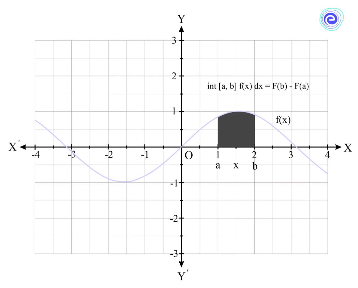
Finding this area requires measuring the integral of \(f(x)\) entering in the upper limit \(b\), and subtracting what you get when you enter in the lower limit \(a\).

Steps to Evaluate the Definite Integral

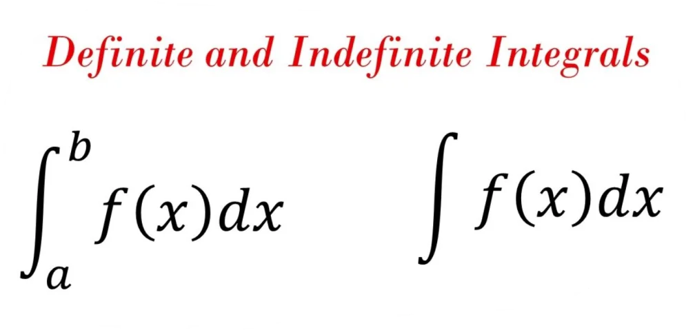
The definite integral of the function \(f(x)\) over the closed interval \([a,\,b]\) is given by \(\int_a^b f (x)dx\) is given below:

• Step 1: Find the indefinite integral \(\int {f(x)} dx\). Let this value be \(F(x)\).
• Step 2: Remove the constant \(C\) (There is no need to keep integration constant \(C\) because if we consider \(F(x) + C\) instead of \(F(x))\)
• Step 3: We get, \(\int_a^b f (x)dx = [F(x) + C]_a^b = [F(b) + C] – [F(a) + C] = F(b) – F(a)\) thus, the arbitrary constant disappears in evaluating the value of the definite integral.
• Step 4: Evaluate \(F(b) – F(a) = [F(x)]_a^b\), which is the value of \(\int_a^b f (x)dx\)

Definite and Indefinite Integrals

In Calculus, the two most significant processes are integration and differentiation. Differentiation is the process of determining a function’s derivative, whereas integration is the process of determining the antiderivative of a function.

The representation of a number that gives a constant result is known as a definite integral. There is always an upper and lower limit to a definite integral. The definite integrals’ limits are constant. A definite integral is sometimes defined as an indefinite integral evaluated over the lower and upper bounds.

Because the value or solution produced by calculating integrals using limits is constant, these integrals are referred to as definite integrals. It is possible for the solution to be either positive or negative. The answer to a defined integral is always in a specific region.

Evaluation as the Limit of Sum

Let \(f(x)\) be a continuous function defined on a closed interval \([a,\,b]\). Assume that all the input values to the function are non-negative, so the graph of the function is a curve above the \(x\)-axis.

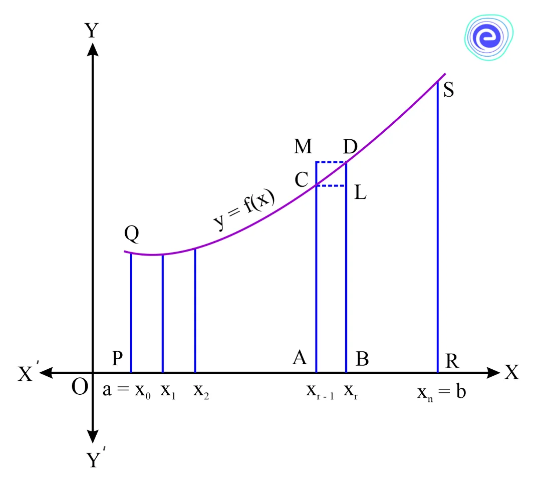
The definite integral \(\int_a^b f (x)dx\) is the area bounded by the curve \(y = f(x)\), the ordinates \(x = a,\,x = b\) and \(x\)-axis the Consider the region \(PRSQP\) between this curve, \(x\)-axis and the ordinates \(x = a\) and \(x = b\), to calculate the area.

Divide the integral \([a,\,b]\) into \(n\) equal subintervals denoted by \(\left[ {{x_0},\,{x_1}} \right],\,\left[ {{x_1},\,{x_2}} \right],\,\left[ {{x_2},\,{x_3}} \right],\, \ldots \ldots \left[ {{x_{r – 1}},\,{x_r}} \right],\, \ldots ..\left[ {{x_{n – 1}},\,{x_n}} \right]\), where \({x_0} = a,\,{x_1} = a + h,\,{x_2} = a + 2h,\, \ldots .{x_r} = a + rh\), and \({x_n} = b = a + nh\).

\(n = \frac{{b – a}}{h}\). Here, as \(n \to \infty ,\,h \to 0\)

The region \(PRSQP\) under consideration Is the sum of subregions, where each subregion is defined on the subintervals \(\left[ {{x_{r – 1}},\,{x_r}} \right],\,r = 1,\,2,\,3,\, \ldots n\)

The area of the region \(ABDCA\) is represented by the sum of all lower and upper rectangles under the curve for the given sub-intervals.

Now, the area is shown by following sum

\({s_n} = h\left[ {f\left( {{x_0}} \right) + \ldots + f\left( {{x_{n – 1}}} \right)} \right ]= h\sum\limits_{r = 0}^{n – 1} f \left( {{x_r}} \right).\)

Symbolically, we can write by using the limits as

\({\log _{n \to \infty }}{S_n} = \) area of the region \(PRSQP = \int_a^b f (x)dx\)

\(\int_a^b f (x)dx = {\log _{h \to \infty }}h[f(a) + f(a + h) + \ldots \ldots .f(a + (n – 1)h]\)

As \(n \to \infty ,\,h = \frac{{b – a}}{n}\), then

\(\int_a^b f (x)dx = (b – a){\log _{n \to \infty }}\frac{1}{n}[f(a) + f(a + h) + \ldots \ldots .f(a + (n – 1)h]\)

This expression gives the evaluation of definite integral as the limit of sum.

Evaluating by Fundamental Theorem of Calculus

By using the second fundamental theorem of Calculus, the definite integral of the curve \(f\left( x \right)\) over the interval \(\left[ {a,\,b} \right]\) is given by

\(\int_a^b f (x)dx = F(b) – F(a)\)

Here, \(F\left( x \right)\) is the integration of the function \(f\left( x \right)\).

Evaluating Using Properties

We can evaluate the definite integral by using the various properties such as:

Property 1: For value of \(‘t’\), such that \(x = t\), we have property is \(\int_a^b f (x)dx = \int_a^b f (t)dt\)

Proof: Let us substitute the variable \(t\) for the given variable \(x\)

\(x = t\)

\( \Rightarrow dx = dt\)

So, \(\int_a^b f (x)dx = \int_a^b f (t)dt\)

Property 2: The sign of the integration will change if we interchange the limits
\(\int_a^b f (x)dx = – \int_b^a f (x)dx\)

Property 3: \(\int_a^b f (x)dx = \int_a^c f (x)dx + \int_c^b f (x)dx\)

Proof: Let \(F\) be anti-derivative of \(f\). Then

\(\int_a^b f (x)dx = F(b) – F(a)\,……(i)\)

\(\int_a^c f (x)dx = F(c) – F(a)\,……(ii)\)

\(\int_c^b f (x)dx = F(b) – F(c)\,……(iii)\)

Adding \((ii)\) and \((iii)\), we get

\(\int_a^c f (x)dx + \int_c^b f (x)dx = F(b) – F(a)\)

Thus, \(\int_a^b f (x)dx = \int_a^c f (x)dx + \int_c^b f (x)dx\)

Property 4: \(\int_a^b f (x)dx = \int_a^b f (a + b – x)dx\)

Proof: Let \(t = a + b – x\), then \(dt = – dx\).

When, \(x = a,\,t = b\) and \(x = b,\,t = a\).

Therefore,

\(\int_a^b f (x)dx = – \int_b^a f (a + b – t)dt\)

\(\int_a^b f (x)dx = \int_a^b f (a + b – t)dt\) (By property \(3\))

\(\int_a^b f (x)dx = \int_a^b f (a + b – x)dx\) (By property \(1\))

Property 5: \(\int_a^a f (x)dx = 0\)

Proof: We know that \(\int_a^b f (x)dx = F(b) – F(a)\)

So, \(\int_a^a f (x)dx = F(a) – F(a) = 0.\)

Property 6: \(\int_0^a f (x)dx = \int_0^a f (a – x)dx\)

Proof: Let \(t = a – x\), then \(dt = – dx\)

When \(x = 0,\,t = a\) and when \(x = a,\,t = 0\).

Therefore,

\(\int_0^a f (x)dx = – \int_a^0 f (a – t)dt\)
\(\int_0^a f (x)dx = \int_0^a f (a – t)dt\)
\(\int_0^a f (x)dx = \int_0^a f (a – x)dx\)

Property 7: \(\int_0^{2a} f (x)dx = \int_0^a f (x)dx + \int_0^a f (2a – x)dx\)

Proof: Using property \(2,\,\int_0^{2a} f (x)dx = \int_0^a f (x)dx + \int_a^{2a} f (x)dx\)

Let \(t = 2a – x\) in the second integral on \({\rm{R}}{\rm{.H}}{\rm{.S}}{\rm{.}}\)

Then, \( – dx = dt\). When \(x = a,\,t = a\) and \(x = 2a,\,t = 0\)

Then, \(\int_0^{2a} f (x)dx = \int_0^a f (x)dx + \left( { – \int_a^0 f (x)dx} \right)\)

\(\int_0^{2a} f (x)dx = \int_0^a f (x)dx + \int_0^a f (2a – t)dt\)

\(\int_0^{2a} f (x)dx = \int_0^a f (x)dx + \int_0^a f (2a – x)dx\)

Property 8: \(\int_0^{2a} f (x)dx = 2\int_0^a f (x)dx\), if \(f(2a – x) = f(x)\)

Proof: From the above property, we know that,

\(\int_0^{2a} f (x)dx = \int_0^a f (x)dx + \int_0^a f (2a – x)dx\)

When, \(f\left( {2a – x} \right) = f\left( {x} \right)\), then,

\(\int_0^{2a} f (x)dx = \int_0^a f (x) \cdot dx + \int_0^a f (x)dx\)

\(\int_0^{2a} f (x)dx = a\int_0^a f (x)dx\)

When \(f(2a – x) = – f(x)\)

\(\int_0^{2a} f (x)dx = \int_0^a f (x) \cdot dx + \int_0^a – f(x)dx\)

\(\int_0^{2a} f (x)dx = \int_0^a f (x)dx – \int_0^a f (x)dx\)

\(\int_0^{2a} f (x)dx = 0\)

Property 9: \(\int_{ – a}^a f (x)dx = 2\int_0^a f (x)dx\), if \(f( – x) = f(x)\) or even function and \(\int_{ – a}^a f (x)dx = 0\), if \(f( – x) = – f(x)\) or odd function.

Proof: From the second property,

\(\int_{ – a}^a f (x)dx = \int_{{-a}}^0 f (x) \cdot dx + \int_0^a f (x)dx\)

Let \(t = – x\), then \(dt = – dx\)

When \(x = – a,\,t = a\) and when \(x = 0,\,t = 0\)

\(\int_{{-a}}^a f (x)dx = – \int_a^0 f (t) \cdot dt + \int_0^a f (x)dx\)

\(\int_{{-a}}^a f (x)dx = \int_0^a f ( – x) \cdot dx + \int_0^a f (x)dx\,……(i)\)

If \(f\) is an even function, then, \(f( – x) = f(x)\)

So, from \((i)\)

\(\int_{ – a}^a f (x)dx = \int_0^a f (x) \cdot dx + \int_0^a f (x)dx\)

\(\int_{ – a}^a f (x)dx = 2\int_0^a f (x) \cdot dx\)

If \(f\) is an odd function, then \(f( – x) = – f(x)\)

\(\int_{ – a}^a f (x)dx = – \int_0^a f (x) \cdot dx + \int_0^a f (x)dx\)

\(\int_{ – a}^a f (x)dx = 0\)

Evaluation by Substitution Method

The substitution method is one of the commonly used methods for evaluating the definite integral.

The steps to be followed to evaluate the definite integrals by substitution method is given as follows:

• Step 1: Consider the integral without limits and substitute \(y = f(x)\) or \(x = g(y)\) to reduce the given integral to a known form.
• Step 2: Integrate the new integrand with respect to the new variable without mentioning the constant of integration.
• Step 3: Resubstitute for the new variable and write the answer in terms of the original variable.
• Step 4: Find the values of answers obtained by substituting the variables as mentioned in the above step for the given limits of integral.
• Step 5: Find the difference between the values at the upper and lower limits.

Evaluation by Geometry

Steps for evaluating the definite integrals are given below:

• Step 1: Identify the portion of the graph corresponding to the definite integral.
• Step 2: Divide the graph into geometric shapes whose areas can be calculated using formulas in elementary geometry.
• Step 3: Find the signed area of each shape. Remember that area above the \(x\)-axis is considered positive, and the area below the \(x\)-axis is considered negative.
• Step 4: Add all the areas found in step \(3\).

The result is the evaluation of the definite integral.

Solved Examples on Evaluation of Definite Integrals

Q.1. Evaluate \(\int_{ – \frac{\pi }{4}}^{\frac{\pi }{4}} {{{\sin }^2}\,} xdx\)
Ans:
We know that, \({\sin ^2}\,x\) is an even function.
Therefore, by the property of definite integrals,
\(\int_{ – \frac{\pi }{4}}^{\frac{\pi }{4}} {{{\sin }^2}} \,xdx = 2\int_0^{\frac{\pi }{4}} {{{\sin }^2}} \,xdx\)
\( = 2\int_0^{\frac{\pi }{4}} {\frac{{1 – \cos \,2x}}{2}} dx\)
\( = \int_0^{\frac{\pi }{4}} {(1 – \cos \,2x)} dx\)
\( = \left[ {x – \frac{1}{2}\sin \,2x} \right]_0^{\frac{\pi }{4}}\)
\( = \left( {\frac{\pi }{4} – \frac{1}{2}\sin \frac{\pi }{2}} \right) – 0\)
\( = \frac{\pi }{4} – \frac{1}{2}\)

Q.2. Evaluate \(\int_0^1 {\frac{{{{\tan }^{ – 1}}\,x}}{{1 + {x^2}}}} dx\)
Ans:
Let \(t = {\tan ^{ – 1}}\,x\), then \(dt = \frac{1}{{1 + {x^2}}}dx\).
When \(x = 0,\,t = 0\) and \(x = 1,\,t = \frac{\pi }{4}\).
Thus, \(x\) varies \(0\) to \(1\) , whereas \(t\) varies from \(0\) to \(\frac{\pi }{4}\).
\(\int_0^1 {\frac{{{{\tan }^{ – 1}}\,x}}{{1 + {x^2}}}} dx = \int_0^{\frac{\pi }{4}} t dt\)
\( = \left[ {\frac{{{t^2}}}{2}} \right]_0^{\frac{\pi }{4}}\)
\( = \frac{1}{2}\left[ {\frac{{{\pi ^2}}}{{16}} – 0} \right]\)
\( = \frac{{{\pi ^2}}}{{32}}\)

Q.3. Evaluate \(\int_{ – 1}^1 {{{\sin }^5}} \,x\,{\cos ^4}\,xdx\)
Ans:
Let \({\sin ^5}\,x\,{\cos ^4}\,xdx = f(x)\)
Here, \(f( – x) = {\sin ^5}( – x){\cos ^4}( – x)dx = – {\sin ^5}\,x\,{\cos ^4}\,xdx\)
So, \(f\left( { – x} \right) = – f\left( x \right)\)
Then, \(f\left( x \right)\) is an odd function.
Therefore, by using the property of the definite integrals
\(\int_{ – a}^a f (x)dx = 0\), when \(f( – x) = – f(x)\)
So, \(\int_{ – 1}^1 {{{\sin }^5}} \,x\,{\cos ^4}\,xdx = 0\)

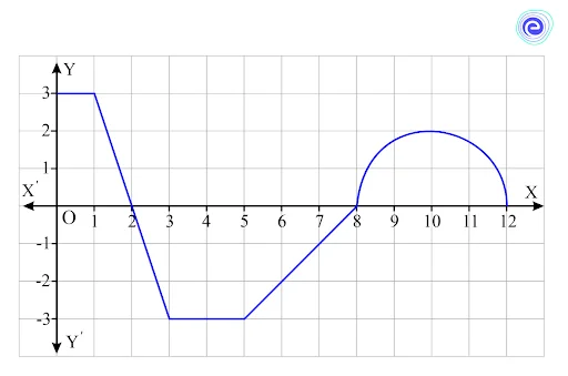
Q.4. Evaluate \(\int_5^{12} f (x)dx\) for the graph given below.

Ans:
Step 1: Identify the portion of the graph corresponding to the definite integral.
Since the definite integral is from \(5\) to \(12\), we only need the portion of the graph between \(x = 5\) and \(x = 12\), shaded below.

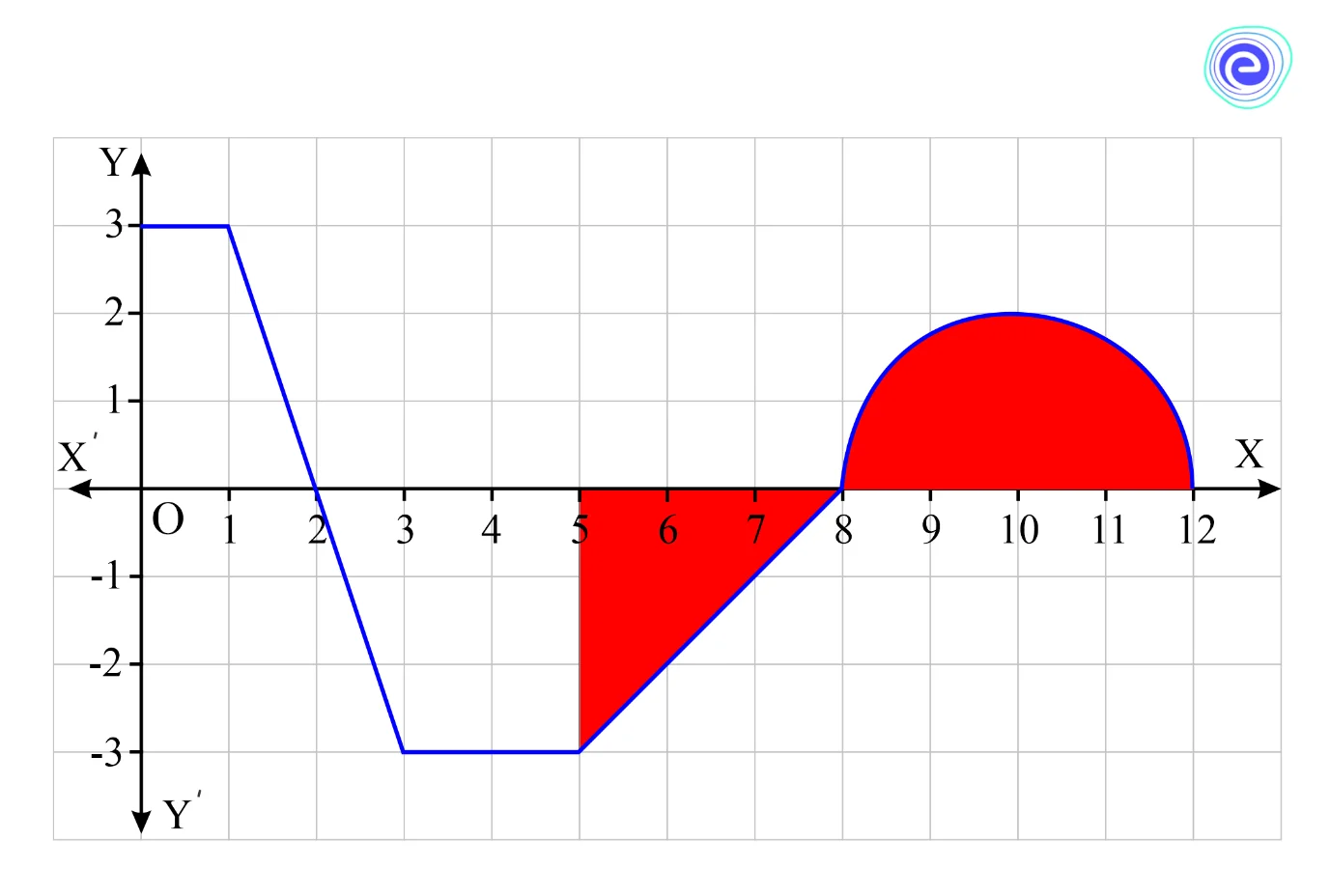
Step 2: Divide the graph into geometric shapes whose areas can be calculated using formulas in elementary geometry.
We can divide this shaded region into a triangle with base \(3\) and \(3\) height and a semicircle with radius \(2\).

Step 3: Find the signed area of each shape. Remember that area above the \(x\)-axis is considered positive, and the area below the \(x\)-axis is considered negative.
The yellow triangle has an area given by

\(A = \frac{1}{2}bh\)

\(A = \frac{1}{2}(3)(3)\)

\(A = \frac{9}{2}\)

Since this area is below the \(x\)-axis, it is counted as negative area. So the area contributed by the yellow triangle is \( – \frac{9}{2}\).
The area of the semicircle with radius \(\)2 is given by

\({\rm{A}} = \frac{1}{2}\pi {r^2}\)

\(A = \frac{1}{2}\pi {(2)^2}\)

\(A = 2\pi \)

This area is considered as a positive area.

Step 4: Add all the areas found in step \(3\). The result is equal to the definite integral.
Using the areas from step \(3\), we have:
\(\int_5^{12} f (x)dx = – \frac{9}{2} + 2\pi \)

Q.5. Evaluate the \(\int_0^1 {\frac{x}{{{x^2} + 1}}} dx\) by using the substitution method.
Ans:
Given: \(\int_0^1 {\frac{x}{{{x^2} + 1}}} dx\)
Let us substitute \({x^2} + 1 = t\)
When \(x = 0,\,t = 1\) and \(x = 1,\,t = 2\)
\( \Rightarrow 2x \cdot \,dx = dt\)
\( \Rightarrow x \cdot dx = \frac{{dt}}{2}\)
So, \(\int_1^2 {\frac{t}{2}} dt\)
\( \Rightarrow \frac{1}{2}[\log \,t]_1^2\)
\( \Rightarrow \frac{1}{2}[\log \,2 – \log \,1]\)
\(\therefore \,\int_0^1 {\frac{x}{{{x^2} + 1}}} dx = \frac{1}{2}\log \,2\)

Summary

Evaluation of definite integral is geometrically finding the area of the curve under a graph with bounded limits. The definite integrals are evaluated by the method of substitution, by using the limit of a sum, using the various properties of definite integrals, and using geometry or graphs. The definite integral is the evaluation of indefinite integral with bounded limits.

Evaluation of a definite integral is the difference of values (integration of indefinite integral) for the upper and lower limits. The definite integral of the curve \(f(x)\) over the interval \([a,\,b]\) is given by \(\int_a^b f (x)dx = F(b) – F(a)\). Here, \(F(x)\) is the integration of the function \(f(x)\).

Frequently Asked Questions (FAQs)

Q.1. What are definite integrals?
Ans: A definite integral defines the area under a curve between two fixed limits. It is represented as \(\int_0^a f (x)dx\), where and are the lower and upper limits, respectively, for a function \(f(x)\), defined with reference to the \(x\)-axis. 

Q.2. How do you evaluate a definite integral?
Ans: Definite integral is evaluated as follows:

• Step 1: Find the integration of indefinite integral.
• Step 2: Apply the limits to the results
• Step 3: Subtract the values obtained by substituting the upper and lower limits.

Q.3. What should be considered first when evaluating definite integrals?
Ans: To evaluate the definite integral, the first thing that we are supposed to do is evaluate the indefinite integral for the function. So, the first thing that should be considered for evaluating the definite integral is to take the indefinite integral and do the integration.

Q.4. How do you evaluate the definite integrals by graph?
Ans: The evaluation of definite integral is finding the area under the curve. To find the area under a curve between two limits, we divide the area into rectangles and sum their areas up. The more the number of rectangles, the more accurate the area is. So we divide the area into an infinite number of rectangles, each with the same (very small) size, and add all the areas.

Q.5. How many ways evaluate the definition integrals?
Ans: Definite integrals are evaluated by different methods. The different methods to evaluate the definite integrals are as follows:

• Fundamental theorem of calculus
• Evaluation of definite integral by substitution
• Evaluation of definite integral by graph
• Evaluation of definite integrals by geometry
• Evaluation of definite integrals by properties

Learn About Applications of Integrals Here

We hope this detailed article on the Evaluation of Definite Integrals will make you familiar with the topic. If you have any inquiries, feel to post them in the comment box. Stay tuned to embibe.com for more information.