Introduction to limit of a function and indeterminate forms: The use of limits in calculus is not limited to finding derivatives and integrals; it has a wide range of applications in other domains. It can be used to measure magnetic, electric fields and to extract the most important data from massive complex functions. The real number system and its distinctive properties require understanding the limit notion. Here, let us learn the meaning of limits and their evaluation with the help of solved examples, in this article.

Introduction to Limit of a Function and Indeterminate Forms

In this article, we will learn what limits and indeterminate forms are, how to determine the existence of limits, evaluation of indeterminate forms and more. We have also included solved examples to give a practical understanding of Introduction to Limit of a Function and Indeterminate Forms.

Informal Approach to Limit

Consider the function, \(f(x) = \frac{{{x^2} – 4}}{{x – 2}}.\) It is defined for all \(x\) except \(x=2,\) as it assumes the form \(\frac{0}{0}\) (indeterminate form).

However, if \(x≠2,\) then \(f(x) = \frac{{(x – 2)(x + 2)}}{{x – 2}} = x + 2\)

The following table exhibits the values of \(f(x)\) at points close to \(2\) on its sides i.e., left and right on the real line.

\(x\)

\(1.4\)

\(1.5\)

\(1.6\)

\(1.7\)

\(1.8\)

\(1.9\)

\(1.99\)

\(2\)

\(2.01\)

\(2.1\)

\(2.2\)

\(2.3\)

\(2.4\)

\(2.5\)

\(f(x)\)

\(3.4\)

\(3.5\)

\(3.6\)

\(3.7\)

\(3.8\)

\(3.9\)

\(3.99\)

\(\frac{0}{0}\)

\(4.01\)

\(4.1\)

\(4.2\)

\(4.3\)

\(4.4\)

\(4.5\)

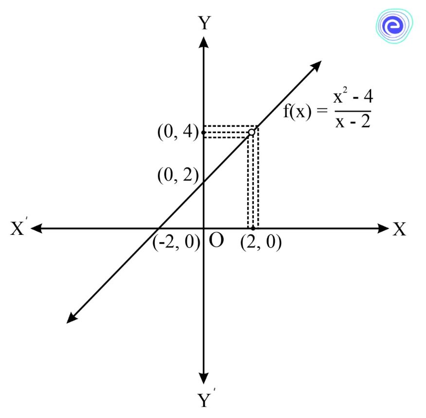
It is evident from the above table and the graph of \(f(x)\) that as \(x\) increases and comes closer to \(2\) from the left-hand side of \(2,\) the values of \(f(x)\) increase and come closer to \(4.\) This is interpreted as,  when \(x\) approaches to \(2\) from its left-hand side, the function \(f(x)\) tends to \(4.\)

Notation for \(‘x\) tends to \(2\) from left-hand side’ is \(x \to {2^ – }.\)

Mathematically, we can write the above explanation as follows:

\(\mathop {\lim }\limits_{x \to {2^ – }} f(x) = 4,\) which means that as \(x\) tends \(2\) to from the left-hand side, the values of\(f(x)\)  tend to \(4.\)

Similarly, we observe from the above table and graph of \(f(x)\) that as \(x\) decreases and comes closer to \(2\) from the right-hand side, the values of \(f(x)\) decrease and come closer to \(4.\)

This is interpreted as, when \(x\) approaches to \(2\) from its right-hand side, the function \(f(x)\) tends to \(4.\)

Notation for \(‘x\) tends to \(2\) from the right-hand side’ is \(x \to {2^ + }.\)

Thus, \(\mathop {\lim }\limits_{x \to {2^+}} f(x) = 4\) means that as \(x\) tends to \(2\) from the right-hand side, the values of \(f(x)\) tend to \(4.\)

Hence, we can approach \(a\) on the real number line either from its left-hand side by increasing numbers less than \(a\) or from the right-hand side by decreasing numbers greater than \(a.\) So, there are two types of limits:

• Left-Hand Limits
• Right-Hand Limits

Existence of Limits

We know that for some functions at \(a,\) the left-hand and right-hand limits are equal, whereas for some functions, these limits are not equal. Sometimes, either the left-hand limit, right-hand limit, or both do not exist.

If \(\mathop {\lim }\limits_{x \to {a^ – }} f(x) = \mathop {\lim }\limits_{x \to {a^ + }} f(x),\) then we say that \(\mathop {\lim }\limits_{x \to a} f(x)\) exists.

Otherwise, \(\mathop {\lim }\limits_{x \to a} f(x)\) does not exist.

Evaluation of Limits

The algorithms for finding the left hand and right-hand limits at \(x=a\) is given as follows

Algorithm for Finding the Left-Hand Limit:

Step 1: Write \(\mathop {\lim }\limits_{x \to {a^ – }} f(x).\)
Step 2: Put \(x=a−ℎ.\)
Step 3: Replace \({x \to {a^ – }}\) by \(ℎ→0\) to obtain \(\mathop {\lim }\limits_{x \to {a^ – }} f(x) = \mathop {\lim }\limits_{h \to 0} f(a – h).\)
Step 4: Simplify \(\mathop {\lim }\limits_{h \to 0} f(a – h)\) by using the formula for the given function.

Algorithm for Finding the Right-Hand Limit:

Step 1: Write \(\mathop {\lim }\limits_{x \to {a^ + }} f(x).\)
Step 2: Put \(x=a+ℎ.\)
Step 3: Replace \({x \to {a^ + }}\) by \(ℎ→0\) to obtain \(\mathop {\lim }\limits_{x \to {a^ + }} f(x) = \mathop {\lim }\limits_{h \to 0} f(a + h).\)
Step 4: Simplify \(\mathop {\lim }\limits_{h \to 0} f(a + h)\) by using the formula for the given function.

Example: Find the left-hand limit and right-hand limit of the function \(f(x) = \left\{ {\begin{array}{*{20}{c}} {\frac{{|x – 4|}}{{x – 4}},}&{x \ne 4}\\ {0,}&{x = 4} \end{array}} \right.\)

Solution: Given: \(f(x) = \left\{ {\begin{array}{*{20}{c}} {\frac{{|x – 4|}}{{x – 4}},}&{x \ne 4}\\ {0,}&{x = 4} \end{array}} \right.\) 

Left-hand limit of \(f(x)\) at \(x=4\)

\( = \mathop {\lim }\limits_{x \to {4^ – }} f(x)\)

\( = \mathop {\lim }\limits_{h \to 0} f(4 – h)\)

\( = \mathop {\lim }\limits_{h \to 0} \frac{{|4 – h – 4|}}{{4 – h – 4}}\)

\( = \mathop {\lim }\limits_{h \to 0} \frac{{| – h|}}{{ – h}}\)

\( = \mathop {\lim }\limits_{h \to 0} \frac{h}{{ – h}}\)

\( = \mathop {\lim }\limits_{h \to 0} ( – 1)\)

Hence, \({\rm{LHL}} = – 1\)

Right hand limit of \(f(x)\) at \(x = 4 = \mathop {\lim }\limits_{x \to {4^ + }} f(x)\)

\( = \mathop {\lim }\limits_{h \to 0} f(4 + h)\)

\( = \mathop {\lim }\limits_{h \to 0} \frac{{|4 + h – 4|}}{{4 + h – 4}}\)

\( = \mathop {\lim }\limits_{h \to 0} \frac{{|h|}}{h}\)

\( = \mathop {\lim }\limits_{h \to 0} \frac{h}{h}\)

\( = \mathop {\lim }\limits_{h \to 0} 1\)

Hence, \({\rm{RHL}} = 1\)

Evaluation of Indeterminate Forms

We know that \(\mathop {\lim }\limits_{x \to a} \frac{{f(x)}}{{g(x)}} = \frac{{\mathop {\lim }\limits_{x \to a} f(x)}}{{\mathop {\lim }\limits_{x \to a} g(x)}},\) provided that \(\mathop {\lim }\limits_{x \to a} g(x) \ne 0,\) and \(\mathop {\lim }\limits_{x \to a} f(x),\) and \(\mathop {\lim }\limits_{x \to a} g(x)\) exists.

If \(\mathop {\lim }\limits_{x \to a} f(x) = \mathop {\lim }\limits_{x \to a} g(x) = 0,\) then \(\mathop {\lim }\limits_{x \to a} \frac{{f(x)}}{{g(x)}}\) takes the form \(\frac{0}{0},\)  which is undefined. But, this does not imply that \(\mathop {\lim }\limits_{x \to a} \frac{{f(x)}}{{g(x)}}\) does not exist. In fact, this limit exists and has a finite value. The determination of limit in such a case is traditionally referred to as the  evaluation of indeterminate form \(\frac{0}{0}.\) There are other types of indeterminate forms, such as: 

• \(\frac{\infty }{\infty }\)
• \(0 \times \infty \)
• \(\infty – \infty \)
• \({0^0}\)
• \({\infty ^0}\)
• \({1^\infty }\)

Among these indeterminate forms \(\frac{0}{0}.\) is fundamental because other forms can easily be reduced to this form.

Methods of Solving \(\frac{0}{0}\) or \(\frac{\infty }{\infty }\) Forms

1. Factorisation Method

If putting \(x=a\) in rational function \(\frac{{f(x)}}{{g(x)}}\) takes the form \(\frac{0}{0}\) or\(\frac{\infty }{\infty },\)  then \(\left( {x – a} \right)\) is a factor of both \(f(x)\) and \(g(x).\)

Hence, to evaluate \(\mathop {\lim }\limits_{x \to a} \frac{{f(x)}}{{g(x)}},\) follow the steps listed below.

Step 1: Factor the numerator and the denominator.

Step 2: Cancel out the common factor \((x−a).\) 

Step 3: Substitute \(x=a\) in the given expression.

Step 4: Repeated the steps till you get a meaningful number.

For example, let us find the value of \(\mathop {\lim }\limits_{x \to – 2} \frac{{{{\left( {{x^2} – x – 6} \right)}^2}}}{{{{(x + 2)}^2}}}.\)

Consider \(\mathop {\lim }\limits_{x \to – 2} \frac{{{{\left( {{x^2} – x – 6} \right)}^2}}}{{{{(x + 2)}^2}}}\)

On substituting \(x=−2\) in the numerator and denominator, we get a \(\frac{0}{0}\) form.

So, we factorise an expression in the numerator and cancel out the common terms in both numerator and denominator.

Thus, \(\mathop {\lim }\limits_{x \to – 2} \frac{{{{\left( {{x^2} – x – 6} \right)}^2}}}{{{{(x + 2)}^2}}} = \mathop {\lim }\limits_{x \to – 2} \frac{{{{(x – 3)}^2}{{(x + 2)}^2}}}{{{{(x + 2)}^2}}}\)

\( = \mathop {\lim }\limits_{x \to – 2} {(x – 3)^2}\)

\( = {( – 2 – 3)^2}\)

\(=25\)

2. Rationalisation Method

This is used when either the numerator, denominator, or both involve an expression with square roots. Substituting the value of \(x,\) the rational expression takes the form \(\frac{0}{0},\) or \(\frac{\infty }{\infty }.\)

For example, evaluate: \(\mathop {\lim }\limits_{x \to 0} \frac{{\sqrt {2 + x} – \sqrt 2 }}{x}.\)

When \(x=0,\) the expression \(\frac{{\sqrt {2 + x} – \sqrt 2 }}{x}\) takes the form \(\frac{0}{0}.\)

Rationalising the numerator, we get 

\(\mathop {\lim }\limits_{x \to 0} \frac{{\sqrt {2 + x} – \sqrt 2 }}{x} = \mathop {\lim }\limits_{x \to 0} \frac{{(\sqrt {2 + x} – \sqrt 2 )(\sqrt {2 + x} + \sqrt 2 )}}{{x(\sqrt {2 + x} + \sqrt 2 )}}\,\,\,\,\left( {{\rm{form }}\frac{0}{0}} \right)\)   

\( = \mathop {\lim }\limits_{x \to 0} \frac{{2 + x – 2}}{{x(\sqrt {2 + x} + \sqrt 2 )}}\)

\( = \mathop {\lim }\limits_{x \to 0} \frac{1}{{\sqrt {2 + x} + \sqrt 2 }} = \frac{1}{{2\sqrt 2 }}\)

3. Some Standard Limits for Evaluation :

Algebraic Limit	If \(n \in Q,\) then \(\mathop {\lim }\limits_{x \to a} \frac{{{x^n} – {a^n}}}{{x – a}} = n{a^{n – 1}}\)
Trigonometric Limits	\((i)\mathop {\lim }\limits_{x \to 0} \frac{{\sin x}}{x} = 1\) \((ii)\mathop {\lim }\limits_{x \to 0} \frac{{\tan x}}{x} = 1\) \((iii)\mathop {\lim }\limits_{x \to 0} \frac{{{{\sin }^{ – 1}}x}}{x} = 1\) \((iv)\mathop {\lim }\limits_{x \to 0} \frac{{{{\tan }^{ – 1}}x}}{x} = 1\) \((v)\mathop {\lim }\limits_{x \to 0} \frac{{\sin {x^0}}}{x} = \frac{\pi }{{180}}\) \((vi)\mathop {\lim }\limits_{x \to 0} \cos x = 1\) \((vii)\mathop {\lim }\limits_{x \to a} \frac{{\sin (x – a)}}{{x – a}} = 1\) \((viii)\mathop {\lim }\limits_{x \to a} \frac{{\tan (x – a)}}{{x – a}} = 1\) \((ix)\mathop {\lim }\limits_{x \to 0} \frac{{1 – \cos x}}{{{x^2}}} = \frac{1}{2}\)
Exponential and Logarithmic Limits	\((i)\mathop {\lim }\limits_{x \to 0} \frac{{{a^x} – 1}}{x} = {\log _e}a,a > 0\) \((ii)\mathop {\lim }\limits_{x \to 0} \frac{{{e^x} – 1}}{x} = 1\) \((iii)\mathop {\lim }\limits_{x \to 0} \frac{{{{\log }_e}(1 + x)}}{x} = 1\) \((iv)\mathop {\lim }\limits_{x \to 0} \frac{{{{\log }_a}(1 + x)}}{x} = \frac{1}{{{{\log }_e}a}},a > 0,a \ne 1\)

4. Evaluation of Limits When Variables Tends to \(∞\) or \(−∞\)

To evaluate this type of limits, follow the steps given below.

Step 1: Write the given expression in the form of a rational function, i.e. \(\frac{{f(x)}}{{g(x)}}.\)
Step 2: If \(k\) is the highest power of \(x\) in numerator and denominator. Then, divide each term in numerator and denominator by \({x^k}.\)
Step 3:  Use the result \(\mathop {\lim }\limits_{x \to \infty } \frac{c}{{{x^n}}} = 0,\) and \(\mathop {\lim }\limits_{x \to \infty } c = c\) where \(n>0\)

For example, evaluate: \(\mathop {\lim }\limits_{x \to \infty } \frac{{a{x^2} + bx + c}}{{d{x^2} + ex + f}}.\)

Here the expression assumes the form \(\frac{\infty }{\infty }.\) Notice that the highest power of \(x\) in both the numerator and denominator is \(2.\) So, we divide each term in both the numerator and  denominator by \({x^2}.\) 

\(\therefore \mathop {\lim }\limits_{x \to \infty } \frac{{a{x^2} + bx + c}}{{d{x^2} + ex + f}} = \mathop {\lim }\limits_{x \to \infty } \frac{{a + \frac{b}{x} + \frac{c}{{{x^2}}}}}{{d + \frac{e}{x} + \frac{f}{{{x^2}}}}}\)

\( = \frac{{a + 0 + 0}}{{d + 0 + 0}}\)

\( = \frac{a}{d}\)

5. Evaluating Limits Using Expansions:

Sometimes, following expansions are helpful in evaluating limits.

\((i)\,{(1 + x)^n} = 1 + nx + \frac{{n(n – 1)}}{{2!}}{x^2} + \frac{{n(n – 1)(n – 2)}}{{3!}}{x^3} + \cdots \)

\((ii){\log _e}(1 + x) = x – \frac{{{x^2}}}{2} + \frac{{{x^3}}}{3} – \frac{{{x^4}}}{4} + \frac{{{x^5}}}{5} \ldots \)

\((iii){\log _e}(1 – x) = – x – \frac{{{x^2}}}{2} – \frac{{{x^3}}}{3} – \frac{{{x^4}}}{4} – \frac{{{x^5}}}{5} \ldots \)

\((iv)\,{e^x} = 1 + x + \frac{{{x^2}}}{{2!}} + \frac{{{x^3}}}{{3!}} + \frac{{{x^4}}}{{4!}} \ldots \)

\((v)\,{e^{ – x}} = 1 – x + \frac{{{x^2}}}{{2!}} – \frac{{{x^3}}}{{3!}} + \frac{{{x^4}}}{{4!}} \cdots \)

\((vi)\,{a^x} = 1 + x\left( {{{\log }_e}a} \right) + \frac{{{x^2}}}{{2!}}{\left( {{{\log }_e}a} \right)^2} + \cdots \)

\((vii)\sin x = x – \frac{{{x^3}}}{{3!}} + \frac{{{x^5}}}{{5!}} – \frac{{{x^7}}}{{7!}} \ldots \)

\((viii)\cos x = 1 – \frac{{{x^2}}}{{2!}} + \frac{{{x^4}}}{{4!}} – \frac{{{x^6}}}{{6!}} \ldots \)

\((ix)\tan x = x + \frac{{{x^3}}}{3} + \frac{2}{{15}}{x^5} + \cdots \)

6. Indeterminate Form and L’hospital’s Rule:

If \(f(x)\) and \(g(x)\) are two functions such that

• \(\mathop {\lim }\limits_{x \to a} f(x) = \mathop {\lim }\limits_{x \to a} g(x) = 0\)
• both are continuous at \(x=a,\)
• both are differential able at \(x=a\)
• \(f'(x)\) and \(g'(x)\) are continuous at the point \(x=a,\) then \(\mathop {\lim }\limits_{x \to a} \frac{{f(x)}}{{g(x)}} = \mathop {\lim }\limits_{x \to a} \frac{{{f^\prime }(x)}}{{{g^\prime }{{(x)}^\prime }}}\) provided \(g(a) \ne 0.\)

Remark:  The L’hospital’s  rule is also applicable if \(\mathop {\lim }\limits_{x \to a} f(x) = \infty \) and \(\mathop {\lim }\limits_{x \to a} g(x) = \infty .\)

Generalisation: If \(\mathop {\lim }\limits_{x \to a} \frac{{{f^\prime }(x)}}{{{g^\prime }(x)}}\) assumes the indeterminate form \(\frac{0}{0}\) and \({f^\prime }(x),{g^\prime }(x)\) satisfy all the conditions described above for \(f(x)\) and \(g(x)\) then  we can repeat the application of this rule on  \(\frac{{{f^\prime }(x)}}{{{g^\prime }(x)}}\) to get

\(\mathop {\lim }\limits_{x \to a} \frac{{f(x)}}{{g(x)}} = \mathop {\lim }\limits_{x \to a} \frac{{{f^{\prime \prime }}(x)}}{{{g^{\prime \prime }}(x)}}\)

Methods of Solving \(∞−∞\) and \(0×∞\) Forms

We know that, \(\mathop {\lim }\limits_{x \to a} (f(x) – g(x))\) is said to be of \(∞−∞\) form if \(f(a) = \infty \) and \(g(a) = \infty .\) And, \(\mathop {\lim }\limits_{x \to a} (f(x) \times g(x))\) is said to be of \(0×∞\) form if \(f(a) = 0\) and \(g(a) = \infty .\)

To solve these two forms, we convert each of these forms to either \(\frac{0}{0}\) or \(\frac{\infty }{\infty }\) form as follows:

• Substitute \(x = \frac{1}{t}\) in form \(\mathop {\lim }\limits_{x \to a} (f(x) – g(x)),\) and then simplify.
• Write \(\mathop {\lim }\limits_{x \to a} (f(x) \times g(x)) = \mathop {\lim }\limits_{x \to a} \frac{{g(x)}}{{\frac{1}{{f(x)}}}}\) or \(\mathop {\lim }\limits_{x \to a} (f(x) \times g(x)) = \mathop {\lim }\limits_{x \to a} \frac{{f(x)}}{{\frac{1}{{g(x)}}}}.\)

Example: Evaluate \(\mathop {\lim }\limits_{x \to \infty } \left( {\sqrt {25{x^2} – 3x} – 5x} \right).\)

Solution: We can see that the given expression is of \(∞−∞\) form.

To solve this expression, we substitute \(x = \frac{1}{t}.\)

Now, \(x→∞⇒t→0\)

\(\therefore \mathop {\lim }\limits_{x \to \infty } \left( {\sqrt {25{x^2} – 3x} – 5x} \right) = \mathop {\lim }\limits_{t \to 0} \left( {\sqrt {\frac{{25}}{{{t^2}}} – \frac{3}{t}} – \frac{5}{t}} \right)\)

\( = \mathop {\lim }\limits_{t \to 0} \left( {\sqrt {\frac{{25 – 3t}}{{{t^2}}}} – \frac{5}{t}} \right)\)

\( = \mathop {\lim }\limits_{t \to 0} \left( {\frac{{\sqrt {25 – 3t} – 5}}{t}} \right)\quad \left( {\frac{0}{0}\,{\rm{form}}} \right)\)

Now, we can apply the method of rationalisation to evaluate the above limit.

\(\therefore \mathop {\lim }\limits_{x \to \infty } \left( {\sqrt {25{x^2} – 3x} – 5x} \right) = \mathop {\lim }\limits_{t \to 0} \left( {\frac{{\sqrt {25 – 3t} – 5}}{t} \times \frac{{(\sqrt {25 – 3t} + 5)}}{{(\sqrt {25 – 3t} + 5)}}} \right)\)

\( = \mathop {\lim }\limits_{t \to 0} \frac{{25 – 3t – 25}}{{t\sqrt {25 – 3t} + 5}}\)

\( = \mathop {\lim }\limits_{t \to 0} \frac{{ – 3t}}{{t\sqrt {25 – 3t} + 5}}\)

\( = \mathop {\lim }\limits_{t \to 0} \frac{{ – 3}}{{\sqrt {25 – 3t} + 5}}\)

\( = \frac{{ – 3}}{{5 + 5}}\)  (Direct Substitution)

Hence, \(\mathop {\lim }\limits_{x \to \infty } \left( {\sqrt {25{x^2} – 3x} – 5x} \right) = – \frac{3}{{10}}\)

Methods of Solving \({0^0},{\infty ^0}\)

These indeterminate forms can be solved as follows:

Consider \(\mathop {\lim }\limits_{x \to a} {(f(x))^{g(x)}}\) is taking any one form among the given forms. To evaluate this limit,

Let \(L = \mathop {\lim }\limits_{x \to a} {(f(x))^{g(x)}}\)

Take logarithm on both sides of the above equation,

\({\log _e}L = {\log _e}\left[ {\mathop {\lim }\limits_{x \to a} {{(f(x))}^{g(x)}}} \right]\)

\( = \mathop {\lim }\limits_{x \to a} \left[ {{{\log }_e}{{(f(x))}^{g(x)}}} \right]\)

\( = \mathop {\lim }\limits_{x \to a} \left[ {g(x){{\log }_e}f(x)} \right]\)

\( \Rightarrow L = {e^{\mathop {\lim }\limits_{x \to a} \left[ {g(x){{\log }_e}f(x)} \right]}}\)

Example: Evaluate : \(\mathop {\lim }\limits_{x \to 0} {x^x}\)

Solution: Let \(y = \mathop {\lim }\limits_{x \to 0} {x^x}\)

Taking natural logarithm on both sides of the equation, we have

\({\log _e}y = {\log _e}\mathop {\lim }\limits_{x \to 0} {x^x}\)

\( = \mathop {\lim }\limits_{x \to 0} {\log _e}{x^x}\)

\( = \mathop {\lim }\limits_{x \to 0} \left[ {x{{\log }_e}x} \right]\,\,\,(0 \times \infty \,{\rm{form}})\)

\( = \mathop {\lim }\limits_{x \to 0} \left[ {\frac{{{{\log }_e}x}}{{\frac{1}{x}}}} \right]\,\,\,\left( {\frac{\infty }{\infty }\,\,{\rm{form}}} \right)\)

\( = \mathop {\lim }\limits_{x \to 0} \frac{{\frac{1}{x}}}{{ – \frac{1}{{{x^2}}}}}\) (L’hospital’s rule)

\( = \mathop {\lim }\limits_{x \to 0} ( – x)\)

\(=0\)

\( \Rightarrow y = {e^0} = 1\)

Hence, \(\mathop {\lim }\limits_{x \to 0} {x^x} = 1\)

Limits of the form, \({1^\infty }\)

In order to evaluate limits of the form \({1^\infty },\) we use the following theorem,

Theorem: If \(f\left( x \right)\) and \(g\left( x \right)\) are two functions such that \(\mathop {\lim }\limits_{x \to a} f(x) = 0 = \mathop {\lim }\limits_{x \to a} g(x),\) then

\(\mathop {\lim }\limits_{x \to a} {[1 + f(x)]^{\frac{1}{{g(x)}}}} = {e^{\mathop {\lim }\limits_{x \to a} \frac{{f(x)}}{{g(x)}}}}\)

Or

If \(\mathop {\lim }\limits_{x \to a} f(x) = 1\) and \(\mathop {\lim }\limits_{x \to a} g(x) = \infty ,\) then \(\mathop {\lim }\limits_{x \to a} {[f(x)]^{g(x)}} = \mathop {\lim }\limits_{x \to a} {[1 + (f(x) – 1)]^{g(x)}} = {{\rm{e}}^{\mathop {\lim }\limits_{x \to a} [f(x) – 1]g(x)}}\)

Particular Cases:

\((i)\mathop {\lim }\limits_{x \to 0} {(1 + x)^{\frac{1}{x}}} = e\)

\((ii)\mathop {\lim }\limits_{x \to \infty } {\left( {1 + \frac{1}{x}} \right)^x} = e\)

\((iii)\mathop {\lim }\limits_{x \to 0} {(1 + \lambda x)^{\frac{1}{x}}} = {e^\lambda }\)

\((iv)\mathop {\lim }\limits_{x \to \infty } {\left( {1 + \frac{\lambda }{x}} \right)^x} = \lambda \)

Solved Examples − Introduction to Limit of a Function and Indeterminate Forms

Q.1. Find the value of \(\mathop {\lim }\limits_{x \to 0} {\left\{ {\frac{{{a^x} + {b^x} + {c^x}}}{3}} \right\}^{\frac{1}{x}}}.\)
Ans: Given: \(\mathop {\lim }\limits_{x \to 0} {\left\{ {\frac{{{a^x} + {b^x} + {c^x}}}{3}} \right\}^{\frac{1}{x}}}\)
\( = \mathop {\lim }\limits_{x \to 0} {\left\{ {1 + \frac{{{a^x} + {b^x} + {c^x} – 3}}{3}} \right\}^{\frac{1}{x}}}\)
\( = \mathop {\lim }\limits_{x \to 0} {\left\{ {1 + \frac{{\left( {{a^x} – 1} \right) + \left( {{b^x} – 1} \right) + \left( {{c^x} – 1} \right)}}{3}} \right\}^{\frac{1}{x}}}\,\,\left( {{1^\infty }\,{\rm{form}}} \right)\)
\( = {e^{\mathop {\lim }\limits_{x \to 0} \left( {\frac{{\left( {{a^x} – 1} \right) + \left( {{b^x} – 1} \right) + \left( {{c^x} – 1} \right)}}{{3x}}} \right)}}\)
\( = {e^{\mathop {\lim }\limits_{x \to 0}\left[ {\frac{{{a^x} – 1}}{{3x}} + \frac{{{b^x} – 1}}{{3x}} + \frac{{{c^x} – 1}}{{3x}}} \right]\)
\( = {e^{\frac{1}{3}\left( {\mathop {\lim }\limits_{x \to 0} \frac{{{a^x} – 1}}{x} + \mathop {\lim }\limits_{x \to 0} \frac{{{b^x} – 1}}{x} + \mathop {\lim }\limits_{x \to 0} \frac{{{c^x} – 1}}{x}} \right)}}\)
\( = {e^{\frac{1}{3}[\log a + \log b + \log c]}}\)
\( = {e^{\log {{(abc)}^{\frac{1}{3}}}}}\)
\( = {(abc)^{\frac{1}{3}}}\)
Hence, \(\mathop {\lim }\limits_{x \to 0} {\left\{ {\frac{{{a^x} + {b^x} + {c^x}}}{3}} \right\}^{\frac{1}{x}}} = {(abc)^{\frac{1}{3}}}\)

Q.2. Evaluate: \(\mathop {\lim }\limits_{x \to \pi } \frac{{1 + {{\sec }^3}x}}{{{{\tan }^2}x}}\)
Ans: Given: \(\mathop {\lim }\limits_{x \to \pi } \frac{{1 + {{\sec }^3}x}}{{{{\tan }^2}x}}\) (\(\left( {\left( {\frac{0}{0}} \right)\) form)
\( = \mathop {\lim }\limits_{x \to \pi } \frac{{\left( {1 + {{\sec }^3}x} \right)}}{{\left( {{{\sec }^2}x – 1} \right)}}\)
\( = \mathop {\lim }\limits_{x \to \pi } \frac{{(\sec x + 1)\left( {{{\sec }^2}x – \sec x + 1} \right)}}{{(\sec x + 1)(\sec x – 1)}}\)
\( = \mathop {\lim }\limits_{x \to \pi } \frac{{{{\sec }^2}x – \sec x + 1}}{{\sec x – 1}}\)
\( = \frac{{1 + 1 + 1}}{{ – 2}}\)
\( = – \frac{3}{2}\)
Hence, \(\mathop {\lim }\limits_{x \to \pi } \frac{{1 + {{\sec }^3}x}}{{{{\tan }^2}x}} = – \frac{3}{2}\)

Q.3. Evaluate: \(\mathop {\lim }\limits_{x \to \frac{\pi }{4}} \frac{{\sin x – \cos x}}{{x – \frac{\pi }{4}}}\)
Ans: Consider \(\mathop {\lim }\limits_{x \to \frac{\pi }{4}} \frac{{\sin x – \cos x}}{{x – \frac{\pi }{4}}}\,\,\,\left( {\left( {\frac{0}{0}} \right)\) form)
\( = \mathop {\lim }\limits_{h \to 0} \frac{{\sin \left( {\frac{\pi }{4} + h} \right) – \cos \left( {\frac{\pi }{4} + h} \right)}}{{\frac{\pi }{4} + h – \frac{\pi }{4}}}\)
\( = \mathop {\lim }\limits_{h \to 0} \frac{{\sin \frac{\pi }{4}\cos h + \cos \frac{\pi }{4}\sin h – \cos \frac{\pi }{4}\cos h + \sin \frac{\pi }{4}\sin h}}{h}\)
\( = \mathop {\lim }\limits_{h \to 0} \frac{{2\left( {\frac{1}{{\sqrt 2 }}\sin h} \right)}}{h}\)
\( = \frac{2}{{\sqrt 2 }}\mathop {\lim }\limits_{h \to 0} \frac{{\sin h}}{h}\)
\( = \sqrt 2 (1)\)
Hence, \(\mathop {\lim }\limits_{x \to \frac{\pi }{4}} \frac{{\sin x – \cos x}}{{x – \frac{\pi }{4}}} = \sqrt 2 \)

Q.4. Evaluate : \(\mathop {\lim }\limits_{x \to – \infty } \left( {\sqrt {{x^2} – x + 1} + x} \right)\)
Ans: We have,
\(\mathop {\lim }\limits_{x \to – \infty } \left( {\sqrt {{x^2} – x + 1} + x} \right) = \mathop {\lim }\limits_{y \to \infty } \left( {\sqrt {{y^2} + y + 1} – y} \right) where \(\y = – {\rm{x}}\)
\( = \mathop {\lim }\limits_{y \to \infty } \frac{{\left\{ {\sqrt {{y^2} + y + 1} – y} \right\}\left\{ {\sqrt {{y^2} + y + 1} + y} \right\}}}{{\left\{ {\sqrt {{y^2} + y + 1} + y} \right\}}}\)
\( = \mathop {\lim }\limits_{y \to \infty } \frac{{{y^2} + y + 1 – {y^2}}}{{\sqrt {{y^2} + y + 1} + y}}\)
\( = \mathop {\lim }\limits_{y \to \infty } \frac{{y + 1}}{{\sqrt {{y^2} + y + 1} + y}}\)
\( = \mathop {\lim }\limits_{y \to \infty } \frac{{1 + \frac{1}{y}}}{{\sqrt {1 + \frac{1}{y} + \frac{1}{{{y^2}}}} + 1}}\)
\( = \frac{1}{2}\)
Hence, \(\mathop {\lim }\limits_{x \to – \infty } \left( {\sqrt {{x^2} – x + 1} + x} \right) = \frac{1}{2}\)

Q.5. Evaluate : \(\mathop {\lim }\limits_{x \to 2} \frac{{x – 2}}{{\sqrt[3]{x} – \sqrt[3]{2}}}\)
Ans: Given: \(\mathop {\lim }\limits_{x \to 2} \frac{{x – 2}}{{\sqrt[3]{x} – \sqrt[3]{2}}} = \mathop {\lim }\limits_{x \to 2} \frac{{x – 2}}{{{x^{\frac{1}{3}}} – {2^{\frac{1}{3}}}}}\)
\( = \frac{1}{{\mathop {\lim }\limits_{x \to 2} \frac{{{x^{\frac{1}{3}}} – {2^{\frac{1}{3}}}}}{{x – 2}}}}\)
\( = \frac{1}{{\frac{1}{3}\left( {{2^{\frac{1}{3} – 1}}} \right)}}\left( {\because \mathop {\lim }\limits_{x \to a} \frac{{{x^n} – {a^n}}}{{x – a}} = n{a^{n – 1}}} \right)\)
\( = \frac{1}{{\frac{1}{3} \times \left( {{2^{^{ – \frac{2}{3}}}}} \right)}}\)
\( = 3\left( {{2^{\frac{2}{3}}}} \right)\)
Hence, \(\mathop {\lim }\limits_{x \to 2} \frac{{x – 2}}{{\sqrt[3]{x} – \sqrt[3]{2}}} = 3\left( {{2^{\frac{2}{3}}}} \right)\)

Summary

In this article we have discussed the Introduction to Limit of a Function and Indeterminate Forms. To summarise all the concepts, there are two types of limits: left-hand and right-hand limits. If \(\mathop {\lim }\limits_{x \to {a^ – }} f(x) = \mathop {\lim }\limits_{x \to {a^ + }} f(x)\) i.e. (LHL at \(x = a\))\(=\)(RHL at \(x = a\)), then we say that \(\mathop {\lim }\limits_{x \to a} f(x)\) exists. Otherwise, \(\mathop {\lim }\limits_{x \to a} f(x)\) does not exist. There are seven types of indeterminate forms such as \(\frac{0}{0},\frac{\infty }{\infty },0 \times \infty ,\infty – \infty ,{0^0},{\infty ^0}\) and \({1^\infty }.\) The most fundamental form among all these is \(\frac{0}{0},\)  and \(\frac{\infty }{\infty }.\) This is because the remaining forms can easily be reduced to \(\frac{0}{0},\)  and \(\frac{\infty }{\infty }.\) form. The various methods like Factorisation, Rationalisation, L’Hospital’s Rule have been explained in this article that are helpful in evaluating all these indeterminate forms.

Frequently Asked Questions (FAQs)

The most commonly asked questions on Introduction to Limit of a Function and Indeterminate Forms are answered below:

Q.1. What is an indeterminate form of a function?
Ans: If on substituting direct limit on given function, we get \(\frac{0}{0},\frac{\infty }{\infty },0 \times \infty ,\infty – \infty ,{0^0},{\infty ^0}\) and \({1^\infty }\) then we cannot evaluate the limits because these are called indeterminate forms.

Q.2. How do you find the limit of the indeterminate form of a function?
Ans: The methods to solve \(\frac{0}{0},\) and \(\frac{\infty }{\infty }.\) forms are
(i) Factorisation Method
(ii) Rationalisation Method
(iii) Solving limits using standard expansions
(iv) Some standard Results.
(v) L’Hospital’s Rule
And, the other forms can be converted to \(\frac{0}{0},\) and \(\frac{\infty }{\infty }.\) forms, and then we can evaluate their limits.

Q.3. What does it mean when a limit is indeterminate?
Ans: An indeterminate form of a limit is one in which the limit of an expression cannot be predicted purely based on the limits of its parts. Instead, more investigation is required to identify the limit and whether or not it exists.

Q.4. What is the difference between undefined and indeterminate?
Ans: Undefined mathematical expressions are those that defy the rules of Mathematics. That is essentially a division by zero. Indeterminate is any mathematical expression that is mathematically correct but cannot be determined using usual procedures. As the variable in both approaches a specific value, a fraction can have a numerator and denominator that approach \(\frac{0}{0}\) or \(\frac{\infty }{\infty }.\)

Q.5.What is an intermediate form in limits?
Ans: Indeterminate refers to an unknown value. The indeterminate form is a mathematical phrase that states that we cannot determine the original value, even after the limits have been substituted.

Q.6.Where can I find a good Introduction to Limit of a Function and Indeterminate Forms?
Ans: You can find the most comprehensive and clear Introduction to Limit of a Function and Indeterminate Forms in this article. For further learning and practice download the embibe app or log in to embibe.com today.

We hope this detailed article on Introduction to Limit of a Function and Indeterminate Forms helps you. If you have any queries, feel to ask in the comment section below and we will get back to you at the earliest.