The Method of Least Squares: We come across variables during time series analysis, and many of them are the dependent type. Determining a relation between two or more variables is frequently required. The method of least squares is used to determine the best fit of a set of data points. The sum of the regressions of points from the plotted curve is minimised. It provides the best-fit trend line. In time series analysis, this method is the most widely used.

The least squares regression is utilised to predict the behaviour of dependent variables. The least squares method is widely used in evaluation and regression. This method is said to be a standard approach in regression analysis for approximating sets of equations with more equations than unknowns. It is associated with regression analysis and is widely used to make scatter plots easier to interpret.

What is the Method of Least Squares?

The method of least squares is a statistical method for determining the best fit line for given data in the form of an equation such as \(y = mx + b.\) The regression line is the curve of the equation. The goal of this method is to minimise the sum of squared errors as much as possible. This method is frequently used in data fitting, where the best fit result is supposed to reduce the sum of squared errors, which is defined as the difference between observed and fitted values. The sum of squared errors helps identify variation in observable data. The method of least squares analysis begins with a set of data points to be plotted on the graph of the \(XY\) plane.

Need for Least Square Method

Regression and evaluation make extensive use of the method of least squares. It is a conventional approach for the least square approximation of a set of equations with unknown variables than equations in the regression analysis procedure.

This method is used as a solution to minimise the sum of squares of all deviations each equation produces. It is commonly used in data fitting to reduce the sum of squared residuals of the discrepancies between the approximated and corresponding fitted values.

Line of Best Fit

The equation that gives the picture of the relationship between the data points is found in the line of best fit. It is calculated by the method of least squares. Computer software models that offer a summary of output values for analysis. The coefficients and summary output values explain the dependence of the variables being evaluated. It can be used to identify the line of best-fit equations.

Least Squares Regression Line

A least squares regression line best fits a linear relationship between two variables by minimising the vertical distance between the data points and the regression line. Since it is the minimum value of the sum of squares of errors, it is also known as “variance,” and the term “least squares” is also used.

On the vertical \(y\)-axis, the dependent variables are plotted, while the independent variables are plotted on the horizontal \(x\)-axis.

Types of Method of Least Squares

The method of least squares problems is divided into two categories. Linear or ordinary least square method and non-linear least square method. These are further classified as ordinary least squares, weighted least squares, alternating least squares and partial least squares.

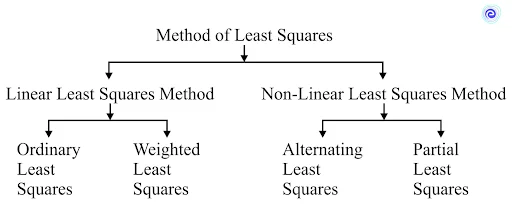
These are dependent on the residuals’ linearity or non-linearity. In statistics, linear problems are frequently encountered in regression analysis. Non-linear problems are commonly used in the iterative refinement method.

Method of Least Squares Graph

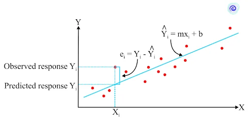
Taking a look at the graph below, the straight line indicates a possible relationship between the independent and dependent variables. This method aims to reduce the gap between the observed response and the regression line’s expected response. The model fits better if there are fewer residuals. This method reduces the residuals of each point from the line that must be used to minimise the data points. There are two types of residuals: vertical and perpendicular. Perpendicular is utilised in general, while vertical is employed largely in polynomials and hyperplane problems, as shown in the graphic below.

Line of Best Fit Equation

The line of best fits gives a set of observations with the least sum of squared residuals, or errors is known as the least-square technique. Assume the data points are \(\left( {{x_1},{x_2}} \right),\left( {{x_2},{y_2}} \right),\left( {{x_3},{y_3}} \right)……,\left( {{x_n},{y_n}} \right),\) with all \(x’s\) being independent variables and all \(y’s\) being dependent variables.
The linear line with the formula \(y = mx + b,\) where \(y\) and \(x\) are variables, \(m\) represents the slope, and \(b\) represents the \(y\)-intercept is found by using this method.
The following is the formula for calculating slope \(m\) and the value of \(b:\) \(m = \frac{{n\sum x y – \sum y \Sigma x}}{{n\sum {{x^2}} – {{\left( {\sum x } \right)}^2}}}\) \(b = \frac{{\sum y – m\sum x }}{n}\). Here, \(n\) is the data points number.

Steps to Find the Line of Best Fit

The steps involved in the method of least squares using the given formulas are as follows.

• Create a table with four columns, the first two of which are for \(x\) and \(y\) coordinates.

• Find \(xy\) and \(\left( {{x^2}} \right)\) in the next two columns.

• Calculate \(\sum x ,\sum y ,\,\sum x y,\) and \({\sum {\left( x \right)} ^2}\)

• Using the formula, calculate the value of slope \(m.\); \(m = \frac{{n\sum x y – \sum y \sum x }}{{n\sum {{x^2}} – {{\left( {\sum x } \right)}^2}}}\)

• Using the formula, find the value of \(b.\); \(b = \frac{{\Sigma y – m\sum x }}{n}\)

• In the equation \(y = mx + b,\) substitute the values of \(m\) and \(b.\)

Limitations of the Method of Least Squares

Even though the method of least squares is regarded as an excellent method for determining the best fit line, it has several drawbacks.

• Only the relationship between the two variables is displayed using this method. None of the other causes or effects is taken into account.
• This approach is unreliable when data is not evenly distributed and is particularly susceptible to outliers. The results of the least squares analysis may be skewed due to this.

Solved Examples – The Method of Least Squares

Below are a few solved examples that can help in getting a better idea.

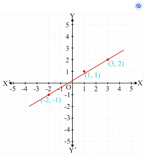
Q.1. Consider the points: \(\left( {1,1} \right),\left( { – 2, – 1} \right)\) and \(\left( {3,2} \right).\) In the same graph, plot these points and the least-squares regression line.
Ans: The value of \(n = 3\)

\(x\)	\(y\)	\(xy\)	\({x^2}\)
\(-2\)	\(-1\)	\(2\)	\(4\)
\(1\)	\(1\)	\(1\)	\(1\)
\(3\)	\(2\)	\(6\)	\(9\)
\(\sum x = 2\)	\(\sum y = 2\)	\(\sum x y = 9\)	\(\sum {{x^2}} = 14\)

Here, \(m = \frac{{n\sum x y – \sum y \sum x }}{{n\sum {{x^2}} – {{\left( {\sum x } \right)}^2}}}\)
\(m = \frac{{\left[ {\left( {3 \times 9} \right) – \left( {2 \times 2} \right)} \right]}}{{3 \times 14 – {2^2}}}\)
\( = \frac{{27 – 4}}{{42 – 4}}\)
\(\therefore m = \frac{{23}}{{38}}\)
\(b = \frac{{\Sigma y – m\sum x }}{n}\)
\(b = \frac{{\left[ {2 – \left( {\frac{{23}}{{38}}} \right) \times 2} \right]}}{3}\)
\( = \frac{{\left[ {2 – \left( {\frac{{23}}{{19}}} \right)} \right]}}{3}\)
\(\therefore b = \frac{5}{{19}}\)
So, the equation least squares regression line is \(y = \frac{{23}}{{38}}x + \frac{5}{{19}}\)
And, graph of the given points and the line of least squares is shown below:

Q.2. Consider the following set of coordinates: \(\left( { – 1,0} \right),\left( {0,2} \right),\left( {1,4} \right),\) and \(\left( {k,5} \right).\) In the equation of least squares, the slope and \(y\)-intercept are \(1.7\) and \(1.9,\) respectively. Can you find the value of \(k\)?
Ans: From the given data, \(n = 4\)
Given:
\(m = 1.7\)
\(b = 1.9\)

\(x\)	\(y\)
\(-1\)	\(0\)
\(0\)	\(2\)
\(1\)	\(4\)
\(k\)	\(5\)
\(\sum x = k\)	\(\sum y = 11\)

\(b = \frac{{\Sigma y – m\Sigma x}}{n}\)
\( \Rightarrow 1.9 = \frac{{11 – 1.7k}}{4}\)
\( \Rightarrow 1.9 \times 4 = 11 – 1.7k\)
\( \Rightarrow 1.7k = 11 – 7.6\)
\( \Rightarrow k = \frac{{3.4}}{{1.7}}\)
\(\therefore k = 2\)

Q.3. The following table shows the sales of a company (in million dollars)

\(x\)	\(2015\)	\(2016\)	\(2017\)	\(2018\)	\(2019\)
\(y\)	\(12\)	\(19\)	\(29\)	\(37\)	\(45\)

Estimate the sales using the regression line in the year \(2020.\)
Ans: From the given data, \(n = 5\)
Let us take \(t = x – 2015\) (\(t\) is the number of years after \(2015\))

\(x\)	\(y\)	\(xy\)	\({x^2}\)
\(0\)	\(12\)	\(0\)	\(0\)
\(1\)	\(19\)	\(19\)	\(1\)
\(2\)	\(29\)	\(58\)	\(4\)
\(3\)	\(37\)	\(111\)	\(9\)
\(4\)	\(45\)	\(180\)	\(16\)
\(\sum x = 10\)	\(\sum y = 142\)	\(\sum x y = 368\)	\(\sum {{x^2}} = 30\)

\(m = \frac{{n\Sigma xy – \Sigma y\Sigma x}}{{n\Sigma {x^2} – {{\left( {\sum x } \right)}^2}}}\)
\(m = \frac{{[\left( {5 \times 368} \right) – \left( {142 \times 10} \right)]}}{{5 \times 30 – {{10}^2}}}\)
\( = \frac{{1840 – 1420}}{{150 – 100}}\)
\( = \frac{{42}}{5}\)
\(\therefore m = 8.4\)
\(b = \frac{{\Sigma y – m\Sigma x}}{n}\)
\(b = \frac{{142 – 8.4 \times 10}}{5}\)
\( = \frac{{142 – 84}}{5}\)
\(\therefore m = 11.6\)
Thus, the least squares equation is \(y\left( t \right) = 8.4t + 11.6\)
From the data, \(t = 2020 – 2015\)
\(\therefore t = 5\)
So, we can write,
\(y\left( 5 \right) = 8.4 \times 5 + 11.6\)
\( = 42 + 11.6\)
\(\therefore y\left( 5 \right) = 53.6\)
Hence, the number of sales is \(53.6\)(million dollars) in \(2020.\)

Q.4. Find the slope by using the method of least squares.

\(x\)	\(0\)	\(1\)	\(2\)	\(3\)	\(4\)
\(y\)	\(2\)	\(3\)	\(5\)	\(4\)	\(6\)

Ans:
From the above data, \(n = 5\)

\(x\)	\(y\)	\(xy\)	\({x^2}\)
\(0\)	\(2\)	\(0\)	\(0\)
\(1\)	\(3\)	\(3\)	\(1\)
\(2\)	\(5\)	\(10\)	\(4\)
\(3\)	\(4\)	\(12\)	\(9\)
\(4\)	\(6\)	\(24\)	\(16\)
\(\sum x = 10\)	\(\sum y = 20\)	\(\sum x y = 49\)	\(\sum {{x^2}} = 30\)

\(m = \frac{{n\Sigma xy – \Sigma y\Sigma x}}{{n\Sigma {x^2} – {{\left( {\Sigma x} \right)}^2}}}\)
\( = \frac{{[\left( {5 \times 49} \right) – \left( {20 \times 10} \right)]}}{{5 \times 30 – {{10}^2}}}\)
\( = \frac{{245 – 200}}{{150 – 100}}\)
\( = \frac{{45}}{{50}}\)
\(\therefore m = 0.9\)

Q.5.Find the intercept of the line of least squares.

\(x\)	\(2\)	\(4\)	\(6\)	\(8\)
\(y\)	\(3\)	\(5\)	\(7\)	\(9\)

Ans:
From the above data, \(n = 4\)

\(x\)	\(y\)	\(xy\)	\({x^2}\)
\(2\)	\(3\)	\(6\)	\(4\)
\(4\)	\(5\)	\(20\)	\(16\)
\(6\)	\(7\)	\(42\)	\(36\)
\(8\)	\(9\)	\(72\)	\(64\)
\(\sum x = 20\)	\(\sum y = 24\)	\(\sum x y = 140\)	\(\sum {{x^2}} = 120\)

Using the formula, \(m = \frac{{n\Sigma xy – \Sigma y\Sigma x}}{{n\Sigma {x^2} – {{\left( {\Sigma x} \right)}^2}}},\) we get
\(m = \frac{{[\left( {4 \times 140} \right) – \left( {20 \times 24} \right)]}}{{4 \times 120 – {{20}^2}}}\)
\( = \frac{{560 – 480}}{{480 – 400}}\)
\( = \frac{{80}}{{80}}\)
\(\therefore m = 1\)
And, \(b = \frac{{\sum y – m\sum x }}{n}\)
\(b = \frac{{24 – 1 \times 20}}{4}\)
\( = \frac{{4}}{{4}}\)
\(\therefore b = 1\)
Hence, the intercept of the line of least squares is \(1.\)

Summary

The method of least squares is a statistical procedure for determining the best fit line for a group of data points by reducing the total of the points’ offsets or residuals from the plotted curve. The method of least squares regression is utilised to predict the behaviour of dependent variables. It explains why the line of best fit should be placed among the data points under consideration. The least squares method is applied in numerous industries, including banking and investment. The best fit line for given data is in the form of an equation such as \(y = mx + b.\) The regression line is the curve of this equation. Although the method is excellent for determining the best fit line, it has several drawbacks too.

FAQs on Method of Least Squares

Students might be having many questions with respect to the Method of Least Squares. Here are a few commonly asked questions and answers.

Q.1. What are the uses of a simple least square method?
Ans: The simple least squares method is used to find the predictive model that best fits the data points.

Q.2. Are least squares the same as linear regression?
Ans: No, linear regression and least squares are not the same. Linear regression is the analysis of statistical data to predict the value of the quantitative variable. The least squares method is used in linear regression to find the predictive model.

Q.3. What is the least square method formula?
Ans: For determining the equation of the line for any data, we use the equation \(y = mx + b.\) The least-square method formula is by finding the value of both \(m\) and \(b\) by using the formulas given below.
● \( m = \frac{{n\sum x y – \sum y \sum x }}{{n\sum {{x^2}} – {{\left( {\sum x } \right)}^2}}}\)
● \( b = \frac{{\sum y – m\sum x }}{n}\)

Q.4. What is the purpose of using the method of least squares?
Ans: When the model residuals are normally distributed with a mean of \(0,\) least squares is used as an equivalent to maximum likelihood.

Q.5. What is the least squares curve fitting?
Ans: The least square method is a method for fitting a curve to the given data. It is one of the techniques for determining the line of best fit for a set of data.

We hope this information about the Method of Least Squares has been helpful. If you have any doubts, comment in the section below, and we will get back to you.

Stay tuned to embibe.com to get the latest information and updates!