Properties of definite integrals: Definite integrals can be used to calculate the area beneath a curve and the area between two curves. They are also used to calculate the volumes of three-dimensional solids. Based on the properties of the solid, there are three methods for calculating volumes: slicing, discs, and washers. If you know the density function of an object, then you can use definite integrals to determine its mass. It can also be used to determine the force exerted on a submerged item in a liquid.

In this article, let’s learn about definite integrals and their properties which will aid us in solving questions based on them.

What is a Definite Integral?

A definite integral represents an area under a curve between two points. An area under the curve \(y = f\left( x \right)\), between \(x = a\) and \(x = b\) is found by integrating \(y = f\left( x \right)\). It is integrated from the lower limit \(x = a\) to the upper limit \(x = b\). It is denoted by \(\int\limits_a^b {f\left( x \right)} \,dx\), also known as the definite integral of \(f\left( x \right)\) over \(\left[ {a,\,b} \right]\).

Fundamental Theorem of Calculus

Let \(\phi \left( x \right)\) be the primitive or anti-derivative of a continuous function \(f\left( x \right)\) defined on \(\left[ {a,\,b} \right]\). Then,
\(\frac{d}{{dx}}\left\{ {\phi \left( x \right)} \right\} = f\left( x \right)\)

The definite integral of \(f\left( x \right)\) over the interval \(\left[ {a,\,b} \right]\) is denoted by \(\int\limits_a^b {f\left( x \right)} \,dx\) and is equal to \(\left[ {\phi \left( b \right) – \phi \left( a \right)} \right]\).
\(\int\limits_a^b {f\left( x \right)} \,dx = \phi \left( b \right) – \phi \left( a \right)\)

Here, the numbers \(a\) and \(b\) are called the limits of integration. While \(a\) is called the lower limit, \(b\) is the upper limit. The interval \(\left[ {a,\,b} \right]\) is called the interval of integration.

Steps to Evaluate a Definite Integral

To evaluate the definite integral \(\int\limits_a^b {f\left( x \right)} \,dx\) of a continuous function \(f\left( x \right)\) defined on \(\left[ {a,\,b} \right]\) we may use the following algorithm.

Step\(1\): Find the indefinite integral \(\int {f\left( x \right)\,dx} \). Let this be \(\phi \left( x \right).\) There is no need to keep the constant of integration.

Step \(2\): Evaluate \(\phi \left( a \right)\) and \(\phi \left( b \right)\).

Step \(3\): Calculate \(\phi \left( b \right) – \phi \left( a \right)\).

The value obtained in step \(3\) is the required value of \(\int\limits_a^b {f\left( x \right)} \,dx\).

Properties of Definite Integrals

There are some fundamental properties of definite integrals which are very useful in evaluating integrals.

Property Number	Statement
Property 1	\(\int\limits_a^b {f\left( x \right)} \,dx = \,\int\limits_a^b {f\left( t \right)} \,d{t}\)
Property 2	\(\int\limits_a^b {f\left( x \right)} \,dx = \, – \int\limits_b^a {f\left( x \right)} \,dx\)
Property 3	\(\int\limits_a^b {f\left( x \right)} \,dx = \int\limits_a^c {f\left( x \right)} \,dx + \,\int\limits_c^b {f\left( x \right)} \,dx\), where \(a < c < b\)
Property 4	\(\int\limits_a^b {f\left( x \right)} \,dx = \, \int\limits_a^b {f\left( {a + b – x} \right)} \,dx\)
Property 5	\(\int\limits_0^a {f\left( x \right)} \,dx = \int\limits_0^a {f\left( {a – x} \right)} \,dx\)
Property 6	\(\int\limits_0^{2a} {f\left( x \right)} \,dx = \int\limits_0^a {f\left( x \right)} \,dx + \,\int\limits_0^a {f\left( {2a – x} \right)} \,dx\, = \int\limits_0^a {\left\{ {f\left( x \right)\, + f\left( {2a – x} \right)} \right\}} dx\)
Property 7	\(\int\limits_0^a {x\,f\left( x \right)} \,dx = \,\frac{a}{2}\int\limits_0^a {f\left( x \right)} \,dx\)
Property 8	\(\int\limits_{ – a}^a {\,f\left( x \right)} \,dx = \,\int\limits_0^a {\left\{ {f\left( x \right) + f\left( { – x} \right)} \right\}} \,dx\)
Property 9	\(\int_{ – a}^a f (x)dx = \left\{ {\begin{array}{*{20}{c}}   {2\int_0^a f (x)dx,}&{{\text{ if }}f(x){\text{ is an even function }}} \\   {0,}&{{\text{ if }}f(x){\text{ is an odd function }}} \end{array}} \right.\)
Property 10	\(\int_0^{2a} f (x)dx = \left\{ {\begin{array}{*{20}{c}}   {2\int_0^a f (x)dx,}&{{\text{ if }}f(2a – x) = f(x)} \\   {0,}&{{\text{ if }}f(2a – x) =  – f(x)} \end{array}} \right.\)

Proofs of Properties

Property \(1\):
Statement: \(\int_a^b f (x)dx = \int_a^b f (t)dt\), i.e. integration is independent of the change of variable.
Proof: Let \(\phi \left( x \right)\) be a primitive of \(f\left( x \right)\) Then,
\(\frac{d}{{dx}}\{ \phi (x)\}  = f(x)\)
\( \Rightarrow \frac{d}{{dt}}\{ \phi (t)\}  = f(t)\)
Hence, \(\int_a^b f (x)dx = [\phi (x)]_a^b = \phi (b) – \phi (a)\)  …..\(\left( i \right)\)
And, \(\int_a^b f (t)dt = [\phi (t)]_a^b = \phi (b) – \phi (a)\)   …….\(\left( ii \right)\)
From \(\left( i \right)\) and \(\left( ii \right)\), we obtain
\(\int_a^b f (x)dx = \int_a^b f (t)dt\)

Property \(2\):
Statement: \(\int_a^b f (x)dx =  – \int_b^a f (x)dx\)  i.e. if the limits of a definite integral are interchanged, then its value changes by minus sign only.
Proof: Let \(\phi \left( x \right)\) be the primitive or anti-derivative of a continuous function \(f\left( x \right)\) defined on \(\left[ {a,\,b} \right]\). Then, according to the fundamental theorem of calculus, we have
\(\int\limits_a^b {f\left( x \right)} \,dx = \phi \left( b \right) – \phi \left( a \right)\)
And, \( – \int_b^a f (x)dx =  – [(\phi (a) – \phi (b)] = \phi (b) – \phi (a)\)
\(\therefore \int_a^b f (x)dx =  – \int_b^a f (x)dx\)

Property \(3\):
Statement: \(\int_a^b f (x)dx = \int_a^c f (x)dx + \int_c^b f (x)dx\), where \(a < c < b\).
Proof: Let  \(\phi \left( x \right)\) be a primitive of \(f\left( x \right)\). Then, using the fundamental theorem, we have
\(\int\limits_a^b {f\left( x \right)} \,dx = \phi \left( b \right) – \phi \left( a \right)\)   ……\(\left( i \right)\)
And, \(\int_a^c f (x)dx + \int_c^b f (x)dx = [\phi (c) – \phi (a)] + [\phi (b) – \phi (c)] = \phi (b) – \phi (a)\) ……..\(\left( ii\right)\)
From \(\left( i \right)\) and \(\left( ii \right)\), we have
\(\int_a^b f (x)dx = \int_a^c f (x)dx + \int_c^b f (x)dx\)

Generalisation: The above property can be generalised into the following form:
\(\int_a^b f (x)dx = \int_a^{{c_1}} f (x)dx + \int_{{c_1}}^{{c_2}} f (x)dx +  \ldots  + \int_{{c_n}}^b f (x)dx\) where \(a < {c_1} < {c_2} < {c_3} \cdots  < {c_{n – 1}} < {c_n} < \,b\).

Property \(4\):
Statement: If \(f\left( x \right)\) is a continuous function defined on \(\left[ {a,\,b} \right]\) then
\(\int_a^b f (x)dx = \int_a^b f (a + b – x)dx\)
Proof: Let \(x = a + b – t\) then \(dx =  – dt\)
Also, \(x = a \Rightarrow t = b\) and \(x = b \Rightarrow t = a\)
\(\therefore \int_a^b f (x)dx =  – \int_b^a f (a + b – t)dt\)
\( \Rightarrow \int_a^b f (x)dx = \int_a^b f (a + b – t)dt\)   [By Property \(2\) ]
\( \Rightarrow \int_a^b f (x)dx = \int_a^b f (a + b – x)dx\)   [By Property \(1\) ]
Hence, \(\int_a^b f (x)dx = \int_a^b f (a + b – x)dx\)

Property \(5\):
Statement: If \(f\left( x \right)\) is a continuous function defined on \(\left[ {0,\,a} \right]\) then \(\int_0^a f (x)dx = \int_0^a f (a – x)dx\).
Proof: Let \(x = a – t\) then \(dx =  – dt\)
Also, \(x = 0 \Rightarrow t = a\), and \(x = a \Rightarrow t = 0\)
\(\therefore \int_0^a f (x)dx =  – \int_a^0 f (a – t)dt\)
\( \Rightarrow \int_0^a f (x)dx = \int_0^a f (a – t)dt\)   [By property \(2\)]
\( \Rightarrow \int_0^a f (x)dx = \int_0^a f (a – x)dx\) [By Property \(1\) ]
Hence, \(\int_0^a f (x)dx = \int_0^a f (a – x)dx\)

Property \(6\):
Statement: If \(f\left( x \right)\) is a continuous function defined on \(\left[ {0,\,2a} \right]\), then
\(\int_0^{2a} f (x)dx = \int_0^a f (x)dx + \int_0^a f (2a – x)dx = \int_0^a {\{ f(} x) + f(2a – x)\} dx\)
Proof: Let \(I = \int_0^{2a} f (x)dx\).
Then,
\(I = \int_0^a f (x)dx + \int_a^{2a} f (x)dx\left[ {\because \int_a^b f (x)dx = \int_a^c f (x)dx + \int_c^b f (x)dx} \right]\)
\( \Rightarrow I = \int_0^a f (x)dx + {I_1},{\text{ where }}{I_1} = \int_a^{2a} f (x)dx\)
Let, \(2a – t = x\). Then, \(dx =  – dt\)
Also, \(x = a \Rightarrow t = a\), and \(x = 2a \Rightarrow t = 0\)
\(\therefore {I_1} = \int_a^{2a} f (x)dx = \int_a^0 f (2a – t)( – dt)\)
\( =  – \int_a^0 f (2a – t)dt\)
\( =   \int_0^a f (2a – t)dt\)
\( = \int_0^a {f\left( {2a – x} \right)dx} \)
Substituting the value of \({I_1}\) in \(\left( i \right)\), we get
\(I = \int_0^a f (x)dx + \int_0^a f (2a – x)dx = \int_0^a {\{ f(} x) + f(2a – x)\} dx\)
\(\therefore \int_0^{2a} f (x)dx = \int_0^a {\{ f(} x) + f(2a – x)\} dx\)

Property \(7\):
Statement: Let \(f\left( x \right)\) be a continuous function of \(x\) defined on \(\left[ {0,\,a} \right]\) such that \(f\left( {a – x} \right)\, = \,f\left( x \right)\).
Then,
\(\int_0^a x f(x)dx = \frac{a}{2}\int_0^a f (x)dx\)
Proof: Let \(I = \int_0^a x f(x)dx\).
Then
\(I = \int_0^a {(a – x)} f(a – x)dx\quad \left[ {{\text{Using}}\int_0^a f (x)dx = \int_0^a f (a – x)dx} \right]\)
\( = \int_0^a {(a – x)} f(x)dx[\because f(a – x) = f(x)]\)
\( = a\int_0^a f (x)dx – \int_0^a x f(x)dx\)
\( = a\int_0^a f (x)dx – I\)
\( \Rightarrow 2I = a\int_0^a f (x)dx\)
Hence, \(I = \frac{a}{2}\int_0^a f (x)dx\)

Property \(8\):
Statement:If \(f\left( x \right)\)  is a continuous function defined on \(\left[ {-a,\,a} \right]\) then
\(\int_{ – a}^a f (x)dx = \int_0^a {\{ f(} x) + f( – x)\} dx\)
Proof: Using additive property \(3\), we obtain
\(\int_{ – a}^a f (x)dx = \int_{ – a}^0 f (x)dx + \int_0^a f (x)dx\) …………\(\left( i \right)\)
Let \(x=-t\).
Then, \(dx =  – dt\).
Also, \(x =  – a \Rightarrow t = a\) and \(x =  0 \Rightarrow t = 0\).
\(\therefore \int_{ – a}^0 f (x)dx = \int_a^0 f ( – t)\left( { – dt} \right)\)
\( =  – \int_a^0 f \left( { – t} \right)\,dt\)
\( = \int_0^a {f\left( { – t} \right)dt} \)  [By property \(2\)]
\( \Rightarrow \int_{ – a}^0 f (x)dx = \int_0^a f ( – x)\,dx\)  [By property \(1\)] ……… \(\left( ii \right)\)
From \(\left( i \right)\) and \(\left( ii \right)\), we get
\(\int_{ – a}^a f (x)dx = \int_0^a f ( – x)dx + \int_0^a f (x)dx\)
\( \Rightarrow \int_{ – a}^a f (x)dx = \int\limits_0^a {\left\{ {f( – x) + f(x)} \right\}dx} \)

Property \(9\):
Statement: If \(f\left( x \right)\) is a continuous function defined on \(\left[ {-a,\,a} \right]\) then
\(\int_{ – a}^a f (x)dx = \left\{ {\begin{array}{*{20}{c}}
  {2\int_0^a f (x)dx,}&{{\text{ if }}f(x){\text{ is an even function }}} \\
  {0,}&{{\text{ if }}f(x){\text{ is an odd function }}}
\end{array}} \right.\)
Proof: Using property \(8\), we obtain
\(\int_{ – a}^a f (x)dx = \int\limits_0^a {\left\{ {f( x) + f( – x)} \right\}dx} \)
\( \Rightarrow \int_{ – a}^a {f\left( x \right)\,dx = \left\{ \begin{gathered}\int_0^a {\left\{ {f(x) + f(x)} \right\}dx\,\,\,\,\,{\text{if}}\,f\left( { – x} \right) = f\left( x \right)}  \hfill \\\int\limits_0^a {\left\{ {f(x) – f(x)} \right\}dx,\,\,\,\,{\text{if}}\,f\left( { – x} \right) =  – f\left( x \right)}  \hfill \\\end{gathered}  \right.} \)
\( \Rightarrow \int_{ – a}^a f (x)dx = \left\{ {\begin{array}{*{20}{c}}
  {2\int_0^a f (x)dx,}&{{\text{ if }}f(x){\text{ is an even function }}} \\
  {0,}&{{\text{ if }}f(x){\text{ is an odd function }}}
\end{array}} \right.\)

Property \(10\):
If \(f\left( x \right)\) is a continuous function defined on \(\left[ {0,\,2a} \right]\), then
\(\int_0^{2a} f (x)dx = \left\{ {\begin{array}{*{20}{c}}
  {2\int_0^a f (x)dx,}&{{\text{ if }}f(2a – x) = f(x)} \\
  {0,}&{{\text{ if }}f(2a – x) =  – f(x)}
\end{array}} \right.\)
Proof: Using Property \(6\), we obtain
\(\int_0^{2a} f (x)dx = \,\int\limits_0^a {\left\{ {f(x) + f(2a – x)} \right\}dx} \)
\( \Rightarrow \int\limits_0^{2a} {f\left( x \right)\,dx = \left\{ \begin{gathered}\int\limits_0^a {\left\{ {f(x) + f(x)} \right\}dx,\,\,\,\,\,{\text{if}}\,f\left( {2a – x} \right) = f\left( x \right)}  \hfill \\\int\limits_0^a {\left\{ {f(x) – f(x)} \right\}dx,\,\,\,\,{\text{if}}\,f\left( {2a – x} \right) =  – f\left( x \right)}  \hfill \\\end{gathered}  \right.} \)
Hence,
\(\int_0^{2a} f (x)dx = \left\{ {\begin{array}{*{20}{c}}
  {2\int_0^a f (x)dx,}&{{\text{ if }}f(2a – x) = f(x)} \\
  {0,}&{{\text{ if }}f(2a – x) =  – f(x)}
\end{array}} \right.\)

Solved Examples – Properties of Definite Integrals

Q.1. Evaluate: \(\int_0^1 {\left| {5x – 3} \right|\,dx} \)
Ans: We know that
\(\left| {5x – 3} \right|\, = \left\{ \begin{gathered}- \left( {5x – 3} \right)\,{\text{when}}\,5x – 3 < 0 \Rightarrow x < \frac{3}{5} \hfill \\5x – 3\,{\text{when}}\,5x – 3 \geqslant 0 \Rightarrow x \geqslant \frac{3}{5}\, \hfill \\\end{gathered}  \right.\)
The graph of \(y = \left| {5x – 3} \right|\) is shown in the figure given below.

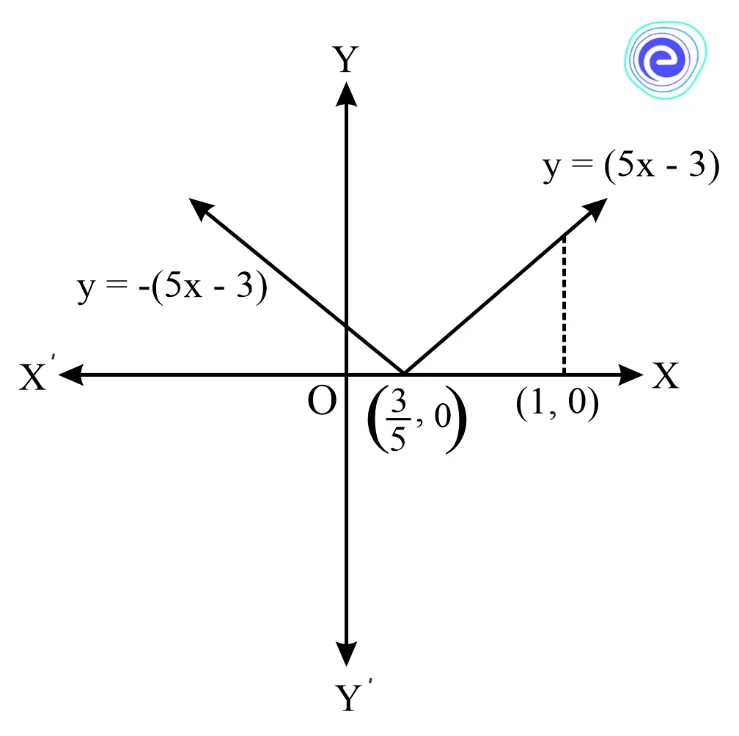
Let \(I = \int\limits_0^1 {\left| {5x – 3} \right|\,dx} \)
Using \(\int\limits_a^b {f\left( x \right)} \,dx = \int\limits_a^c {f\left( x \right)} \,dx + \,\int\limits_c^b {f\left( x \right)} \,dx,\) where \({\text{a}}\,{\text{ < }}\,{\text{c}}\,{\text{ < }}\,{\text{b}}\).
\( = \int\limits_0^{\frac{3}{5}} {\left| {5x – 3} \right|\,dx} \, + \,\int\limits_{\frac{3}{5}}^1 {\left| {5x – 3} \right|\,dx} \)
\( = \int\limits_0^{\frac{3}{5}} { – \left( {5x – 3} \right)\,dx} \, + \,\int\limits_{\frac{3}{5}}^1 {\left( {5x – 3} \right)\,dx} \)
\( = \left[ {3x – 5 \times \frac{{{x^2}}}{2}} \right]_0^{\frac{3}{5}}\, + \,\left[ {\frac{{5{x^2}}}{2} – 3x} \right]_{\frac{3}{5}}^1\)
\( = \left( {\frac{9}{5} – \frac{9}{{10}}} \right) + \,\left( { – \frac{1}{2} + \frac{9}{{10}}} \right)\)
\( = \frac{{13}}{{10}}\)

Q.2. Evaluate \(\int_0^\pi  {\left| {\cos x} \right|\,dx} \)
Ans: We know that
\(\left| {\cos \,x} \right|\, = \left\{ \begin{gathered}\cos \,x\,{\text{when}}\,0 \leqslant x \leqslant \frac{\pi }{2} \hfill \\- \cos \,x\,{\text{when}}\,\frac{\pi }{2} \leqslant x \leqslant \pi \, \hfill \\\end{gathered}  \right.\)
Let \( I = \int_0^\pi  {\left| {\cos x} \right|\,dx} \)
Using additive property, we get
\(I = \int\limits_0^{\frac{\pi }{2}} {\left| {\cos \,x} \right|\,dx\, + } \,\int\limits_{\frac{\pi }{2}}^\pi  {\left| {\cos \,x} \right|\,dx\,} \)
\( = \int\limits_0^{\frac{\pi }{2}} {\cos \,x\,dx\, + } \,\int\limits_{\frac{\pi }{2}}^\pi  {\left( { – \cos \,x} \right)\,dx\,} \)
\( = \left[ {\sin \,x} \right]_0^{\frac{\pi }{2}} – \,\left[ {\sin \,x} \right]_{\frac{\pi }{2}}^0 = 1 + 1 = 2\)

Q.3. Evaluate  \(\int\limits_{ – \frac{\pi }{2}}^{\frac{\pi }{2}} {\frac{{x\,\sin \,x}}{{{e^x} + 1}}\,dx} \)
Ans: Let \(I = \int\limits_{ – \frac{\pi }{2}}^{\frac{\pi }{2}} {\frac{{x\,\sin \,x}}{{{e^x} + 1}}\,dx} \)       ……\(\left( i \right)\)
\( = \int\limits_{ – \frac{\pi }{2}}^{\frac{\pi }{2}} {\frac{{\left( { – \frac{\pi }{2} + \frac{\pi }{2} – x} \right)\sin \,\left( { – \frac{\pi }{2} + \frac{\pi }{2} – x} \right)\,}}{{{e^{\left( { – \frac{\pi }{2} + \frac{\pi }{2} – x} \right)}} + 1}}\,dx} \) [Using \(\int_a^b f (x)dx = \int_a^b f (a + b – x)\,dx\)]
\( \Rightarrow I = \int\limits_{ – \frac{\pi }{2}}^{\frac{\pi }{2}} {\frac{{ – x\,\sin \,\left( { – x} \right)}}{{{e^{ – x}} + 1}}\,dx} \)
\( = \int\limits_{ – \frac{\pi }{2}}^{\frac{\pi }{2}} {\frac{{ x\,\sin \,x\,{e^x}}}{{{e^{ x}} + 1}}\,dx} \) ……….. \(\left( ii\right)\)
Adding \(\left( i\right)\) and \(\left( ii\right)\), we obtain
\(2I = \int\limits_{ – \frac{\pi }{2}}^{\frac{\pi }{2}} {\left( {\frac{{x\,\sin \,x}}{{{e^x} + 1}}\, + \,\frac{{x\,\sin \,x\,{e^x}}}{{{e^x} + 1}}\,} \right)\,dx} \)
\( \Rightarrow 2I = \int\limits_{ – \frac{\pi }{2}}^{\frac{\pi }{2}} {\,x\,\sin \,x\left( {\frac{{{e^x} + 1}}{{{e^x} + 1}}\,\,} \right)\,dx} \)
\( = \int\limits_{ – \frac{\pi }{2}}^{\frac{\pi }{2}} {\,x\,\sin \,x\,dx} \)
\( \Rightarrow 2I~ = ~[ – x\,\cos \,x]_{ – \pi /2}^{\pi /2} + \mathop \smallint \nolimits_{ – \frac{\pi }{2}}^{\frac{\pi }{2}} \cos \,x\,dx\)
\( = [ – x\,\cos \,x]_{ – \frac{\pi }{2}}^{\frac{\pi }{2}} + [\sin \,x]_{ – \pi /2}^{ \pi /2}\)
\( = \left( {0 – 0} \right) + 1 – \left( { – 1} \right)\)
Hence, \(I=1\)

Q.4. Evaluate \(\int\limits_0^{\frac{\pi }{2}} {\frac{{\sqrt {\sin \,x} }}{{\sqrt {\sin \,x} \, + \sqrt {\cos \,x} }}} \,dx\)
Ans: Let \(I=\int\limits_0^{\frac{\pi }{2}} {\frac{{\sqrt {\sin \,x} }}{{\sqrt {\sin \,x} \, + \sqrt {\cos \,x} }}} \,dx\) ……\(\left( i\right)\)
\( = \int\limits_0^{\frac{\pi }{2}} {\frac{{\sqrt {\sin \,\left( {\frac{\pi }{2} – x} \right)} }}{{\sqrt {\sin \,\left( {\frac{\pi }{2} – x} \right)} \, + \sqrt {\cos \,\left( {\frac{\pi }{2} – x} \right)} }}} \,dx\) [Using: \(\int_0^a f (x)dx = \int_0^a f (a – x)\,dx\)]
\( \Rightarrow I = \int\limits_0^{\frac{\pi }{2}} {\frac{{\sqrt {\cos \,x} }}{{\sqrt {\cos \,x} \, + \sqrt {\sin \,x} }}} \,dx\) …….\(\left( ii\right)\)
Adding \(\left( i\right)\) and \(\left( ii\right)\) , we have
\(2I = \int\limits_0^{\frac{\pi }{2}} {\frac{{\sqrt {\sin \,x} }}{{\sqrt {\cos \,x} \, + \sqrt {\sin \,x} }}} \,dx\, + \,\int\limits_0^{\frac{\pi }{2}} {\frac{{\sqrt {\cos \,x} }}{{\sqrt {\sin \,x} \, + \sqrt {\cos \,x} }}} \,dx\)
\( = \int\limits_0^{\frac{\pi }{2}} {\frac{{\sqrt {\sin \,x} \, + \,\sqrt {\cos \,x} }}{{\sqrt {\sin \,x} \, + \sqrt {\cos \,x} }}} \,dx\)
\( = \int\limits_0^{\frac{\pi }{2}} {1.} \,dx\)
\( = \left[ x \right]_0^{\frac{\pi }{2}}\)
\( = \frac{\pi }{2} – 0\)
Hence, \(I = \frac{\pi }{4}\)

Q.5. Evaluate :\(\int\limits_{ – \frac{\pi }{2}}^{\frac{\pi }{2}} {\frac{{1\,\,}}{{1\, + {e^{\sin \,x}}}}\,dx} \)
Ans: Let \( I = \int\limits_{ – \frac{\pi }{2}}^{\frac{\pi }{2}} {\frac{{1\,\,}}{{1\, + {e^{\sin \,x}}}}\,dx} \).
Then,
\(I = \int\limits_0^{\frac{\pi }{2}} {\frac{{1\,\,}}{{1\, + {e^{\sin \,x}}}}\, + \,\frac{{1\,\,}}{{1\, + {e^{ – \sin \,x}}}}\,dx} \,\left[ {\because \,\int\limits_{ – a}^a {f\left( x \right)\,dx = \,\int\limits_0^a {\left\{ {f\left( x \right) + f\left( { – x} \right)} \right\}\,dx} } } \right]\)
\( = \int\limits_0^{\frac{\pi }{2}} {\left\{ {\frac{{1\,\,}}{{1\, + {e^{\sin \,x}}}}\, + \,\frac{{{e^{\sin \,x}}\,\,}}{{1\, + {e^{\sin \,x}}}}} \right\}\,dx} \)
\( = \int\limits_0^{\frac{\pi }{2}} {\frac{{1\, + \,{e^{\sin \,x}}}}{{1\, + {e^{\sin \,x}}}}\,\,\,dx} \)
\( = \int\limits_0^{\frac{\pi }{2}} 1 \,dx\)
\( = \left[ x \right]_0^{\frac{\pi }{2}}\)
\( = \frac{\pi }{2}\)
Hence, \(\int\limits_{ – \frac{\pi }{2}}^{\frac{\pi }{2}} {\frac{{1\,}}{{1\, + {e^{\sin \,x}}}}\,\,\,dx} \, = \frac{\pi }{2}\)

Summary

A definite integral represents an area under a curve between two points. The area under a curve \(y = f\left( x \right)\), between \(x=a\) and \(x=b\) is found by integrating \(y = f\left( x \right)\) from the lower limit \(x=a\) to the upper limit \(x=b\), and it is denoted by \(\int\limits_a^b {f\left( x \right)} \,dx\). There are various properties of definite integral among them the most important properties are \(\int\limits_a^b {f\left( x \right)} \,dx = \, – \int\limits_b^a {f\left( x \right)} \,dx\,,\,\int\limits_a^b {f\left( x \right)} \,dx\, = \,\int\limits_a^b {f\left( {a + b – x} \right)} \,dx,\,\int\limits_{ – a}^a {f\left( x \right)} \,dx\, = \int\limits_0^a {\left\{ {f\left( x \right) + f\left( { – x} \right)} \right\}} \,dx,\), and \(\int_{ – a}^a f (x)dx = \left\{ {\begin{array}{*{20}{c}}
  {2\int_0^a f (x)dx,}&{{\text{ if }}f(x){\text{ is an even function }}} \\
  {0,}&{{\text{ if }}f(x){\text{ is an odd function }}}
\end{array}} \right.\).
It is advised to learn all these properties because they help us find the complex values of some definite integrals.

Frequently Asked Questions (FAQs)

Q.1. Define definite integral?
Ans: A definite integral represents an area under a curve between two points. An area under the curve \(y = f\left( x \right)\), between \(x=a\) and \(x=b\) is found by integrating \(y = f\left( x \right)\) from the lower limit \(x=a\) to the upper limit \(x=b\), and it is denoted by \(\int\limits_a^b {f\left( x \right)} \,dx\), which is also known as a definite integral of \(f\left( x \right)\) over \(\left[ {a,\,b} \right]\).

Q.2. What are the \(6\),\(7\), and \({8^{th}}\) properties of definite integrals?
Ans: Property \(6\): If \(f\left( x \right)\) is a continuous function defined on \(\left[ {0,\,2a} \right]\), then
\(\begin{gathered} \int\limits_0^{2a} {f\left( x \right)} \,dx = \,\int\limits_0^a {f\left( x \right)} \,dx\, + \,\int\limits_0^a {f\left( {2a – x} \right)} \,dx\, = \,\int\limits_0^a {\left\{ {f\left( x \right) + f\left( {2a – x} \right)} \right\}} \,dx \\\end{gathered} \)
Property \(7\): Let \(f\left( x \right)\) be a continuous function of \(x\) defined on \(\left[ {0,\,a} \right]\) such that \(f\left( {a – x} \right) = f\left( x \right)\).
Then,
\(\int\limits_0^a {x\,f\left( x \right)\,dx = \frac{a}{2}} \,\int\limits_0^a {f\left( x \right)} \)
Property \(8\): If \(f\left( x \right)\) is a continuous function defined on \(\left[ {-a,\,a} \right]\) then,
\(\int\limits_{ – a}^a {\,f\left( x \right)\,dx = } \,\int\limits_0^a {\left\{ {f\left( x \right) + f\left( { – x} \right)} \right\}\,dx} \)

Q.3. What are the applications of definite integral?
Ans: Few applications of definite integrals are as follows:
1. Definite integrals can be used to find the area under a curve and the area between two curves.
2. Volumes of three-dimensional solids can find out using the definite integrals.
3. Using a definite integral, we calculate the arc length of a curve.
4. Integrating a force function can also be used to determine work.
5. The force exerted on an object submerged in a liquid can also be calculated using definite integrals

Q.4. What are the different properties of definite integral?
Ans: The different properties of definite integral are as follows:
1. \(\int\limits_a^b {f\left( x \right)\,dx\, = \int\limits_a^b {f\left( t \right)\,dt} } \)
2. \(\int\limits_a^b {f\left( x \right)} \,dx = \, – \int\limits_b^a {f\left( x \right)} \,dx\)
3. \(\int\limits_a^b {f\left( x \right)} \,dx = \int\limits_a^c {f\left( x \right)} \,dx + \,\int\limits_c^b {f\left( x \right)} \,dx,\) where \({\text{a}}\,{\text{ < }}\,{\text{c}}\,{\text{ < }}\,{\text{b}}\).
4. if \(f\left( x \right)\) is a continuous function defined on \(\left[ {a,\,b} \right]\) then
\(\int\limits_a^b {f\left( x \right)} \,dx = \, \int\limits_a^b {f\left( {a + b – x} \right)} \,dx\)
5. If  \(f\left( x \right)\) is a continuous function defined on \(\left[ {0,\,a} \right]\) then
\(\int\limits_0^b {f\left( x \right)} \,dx = \, – \int\limits_0^a {f\left( {a – x} \right)} \,dx\)
6. If \(f\left( x \right)\) is a continuous function defined on \(\left[ {0,\,2a} \right]\), then
\(\int\limits_0^{2a} {f\left( x \right)} \,dx = \int\limits_0^a {f\left( x \right)} \,dx + \,\int\limits_0^a {f\left( {2a – x} \right)} \,dx\, = \int\limits_0^a {\left\{ {f\left( x \right)\, + f\left( {2a – x} \right)} \right\}} dx\)
7. Let \(f\left( x \right)\) be a continuous function of \(x\) defined on \(\left[ {0,\,a} \right]\) such that \(f\left( {a – x} \right) = f\left( x \right)\) Then,
\(\int\limits_0^a {x\,f\left( x \right)\,dx = \frac{a}{2}} \,\int\limits_0^a {f\left( x \right)} \)
8. If \(f\left( x \right)\) is a continuous function defined \(\left[ {-a,\,a} \right]\) on  then
\(\int\limits_{ – a}^a {\,f\left( x \right)\,dx = } \,\int\limits_0^a {\left\{ {f\left( x \right) + f\left( { – x} \right)} \right\}\,dx} \)
9. If \(f\left( x \right)\) is a continuous function defined on \(\left[ {-a,\,a} \right]\) then
\(\int_{ – a}^a f (x)dx = \left\{ {\begin{array}{*{20}{c}}
  {2\int_0^a f (x)dx,}&{{\text{ if }}f(x){\text{ is an even function }}} \\
  {0,}&{{\text{ if }}f(x){\text{ is an odd function }}}
\end{array}} \right.\)
10. 1. If \(f\left( x \right)\) is a continuous function defined on \(\left[ {0,\,2a} \right]\), then
\(\int_0^{2a} f (x)dx = \left\{ {\begin{array}{*{20}{c}}
  {2\int_0^a f (x)dx,}&{{\text{ if }}f(2a – x) = f(x)} \\
  {0,}&{{\text{ if }}f(2a – x) =  – f(x)}
\end{array}} \right.\)

Q.5. What is the value of the definite integral?
Ans: Let \(\phi \left( x \right)\) be the primitive or anti-derivative of a continuous function \(f\left( x \right)\) defined on\(\left[ {a,\,b} \right]\). Then the definite integral of \(f\left( x \right)\) over \(\left[ {a,\,b} \right]\) is denoted by \(\int\limits_a^b {f\left( x \right)\,dx} \) and is equal to \(\left[ {\phi \left( b \right) – \phi \left( a \right)} \right]\).

Learn about Application of Integrals

We hope this detailed article on Properties of Definite Integrals was helpful. If you have any doubts, let us know about them in the comment section below. Our team will get try to solve your queries at the earliest.