Successive differentiation: The higher-order differential coefficients are of utmost importance in scientific and engineering applications. Let \(y=f(x)\) be a function of \(x.\) Then the result of differentiating \(y\) with respect to \(x\) is defined as the derivative or the first derivative of \(y\) with respect to \(x,\) and it is denoted by \(\frac{{dy}}{{dx}}.\) Then, the result of differentiating \(f'(x)\) with respect to \(x\) is defined as the second derivative of the function and it is denoted as \(\frac{{{d^2}y}}{{d{x^2}}}.\)

This process can be defined to \(n\) times, known as successive differentiation. Successive differentiation is the process of differentiating a given function several times, and the results are called successive derivatives. In this article, let us learn more about successive differentiation.

Derivative of a Function

The derivative of \(y=f(x)\) of a variable \(x\) is the measure of the rate at which the value \(y\) of the function changes with respect to the change of the variable \(x.\) It is called the derivative of \(f(x)\) with respect to \(x.\)

Let \(f(x)\) be a function whose domain consists of those values of \(x\) such that the following limit exists.

\(\begin{gathered} {f^\prime }(x) = \mathop {\lim }\limits_{h \to 0} \frac{{f(x + h) – f(x)}}{h} \hfill \\ \hfill \\ \end{gathered} \)

Standard Differentiation Formula

(i) \(\frac{d}{{dx}}(c) = 0,\) where \(c\) is constant

(ii) \(\frac{d}{{dx}}(x) = 1\)

(iii) \(\frac{d}{{dx}}(cx) = c,\) where \(c\) is constant

(iv) \(\frac{d}{{dx}}{x^n} = n{x^{n – 1}},\) power rule

(v) \(\frac{d}{{dx}}{[f(x)]^n} = n{[f(x)]^{n – 1}}{f^\prime }(x),\)

(vi) \(\frac{d}{{dx}}[f(x) + g(x)] = \frac{d}{{dx}}f(x) + \frac{d}{{dx}}g(x)\), sum rule

(vii) \(\frac{d}{{dx}}[f(x) – g(x)] = \frac{d}{{dx}}f(x) – \frac{d}{{dx}}g(x),\) difference rule

(viiii) \(\frac{d}{{dx}}[f(x)g(x)] = f(x)\frac{d}{{dx}}g(x) + g(x)\frac{d}{{dx}}f(x),\) product rule

(ix) \(\frac{d}{{dx}}\left[ {\frac{{f(x)}}{{g(x)}}} \right] = \frac{{g(x)\frac{d}{{dx}}f(x) – f(x)\frac{d}{{dx}}g(x)}}{{{{[g(x)]}^2}}},\) quotient rule

Suppose we want to differentiate the given function twice, thrice, or more. What will happen to the function? Is the result going to be changed?

Chain of Differentiation

Let \(y=x^5\)

For first differentiation \({f^\prime }(x) = 5{x^4}\)

For second differentiation \({f^{\prime \prime }}(x) = 5 \times 4{x^3} = 20{x^3}\)

For third differentiation \({f^{\prime \prime \prime }}(x) = 5 \times 4 \times 3{x^2} = 60{x^2}\)

For fourth differentiation \({f^{iv}}(x) = 5 \times 4 \times 3 \times 2x = 120x\)

For fifth differentiation \({f^v}(x) = 5 \times 4 \times 3 \times 2 \times 1 = 120\)

For sixth differentiation  \({f^{vi}}(x) = 0\)

What is Successive Differentiation?

Successive differentiation is the differentiation of a function successively to derive its higher-order derivatives.

1. If \(y=f(x)\) is a function of \(x,\) then the derivative of \(y\) with respect to \(x\) is denoted by \(\frac{{dy}}{{dx}}\) or \(Dy\) or \(f'(x)\) or \(y_1.\) This is the first-order derivative of \(y.\)
2. If \(\frac{{dy}}{{dx}}\) is differentiated again, \(y=f(x)\) is derivable twice with respect to \(x,\) then the derivative of \(\frac{{dy}}{{dx}}\) with respect to \(x\) is denoted by \(\frac{{{d^2}y}}{{d{x^2}}}\) or \(D^2y\) or \(f^{\prime \prime }(x)\) or \(y_2.\) This is the second-order derivative of \(y.\)
3. If \(\frac{{{d^2}y}}{{d{x^2}}}\) is differentiated again, \(y=f(x)\) is derivable thrice with respect to \(x,\) then the derivative of \(\frac{{{d^2}y}}{{d{x^2}}}\) with respect to \(x\) is denoted by \(\frac{{{d^3}y}}{{d{x^3}}}\) or \(D^3y\) or \(f^{\prime \prime \prime } (x)\) or \(y_3.\) This is called the third-order derivative of \(y.\)

Similarly, we can find the consecutive derivatives, and, in general, the \(n^{th}\) derivative of \(y,\) is obtained by differentiating the given function \(n\) times with respect to \(x.\)

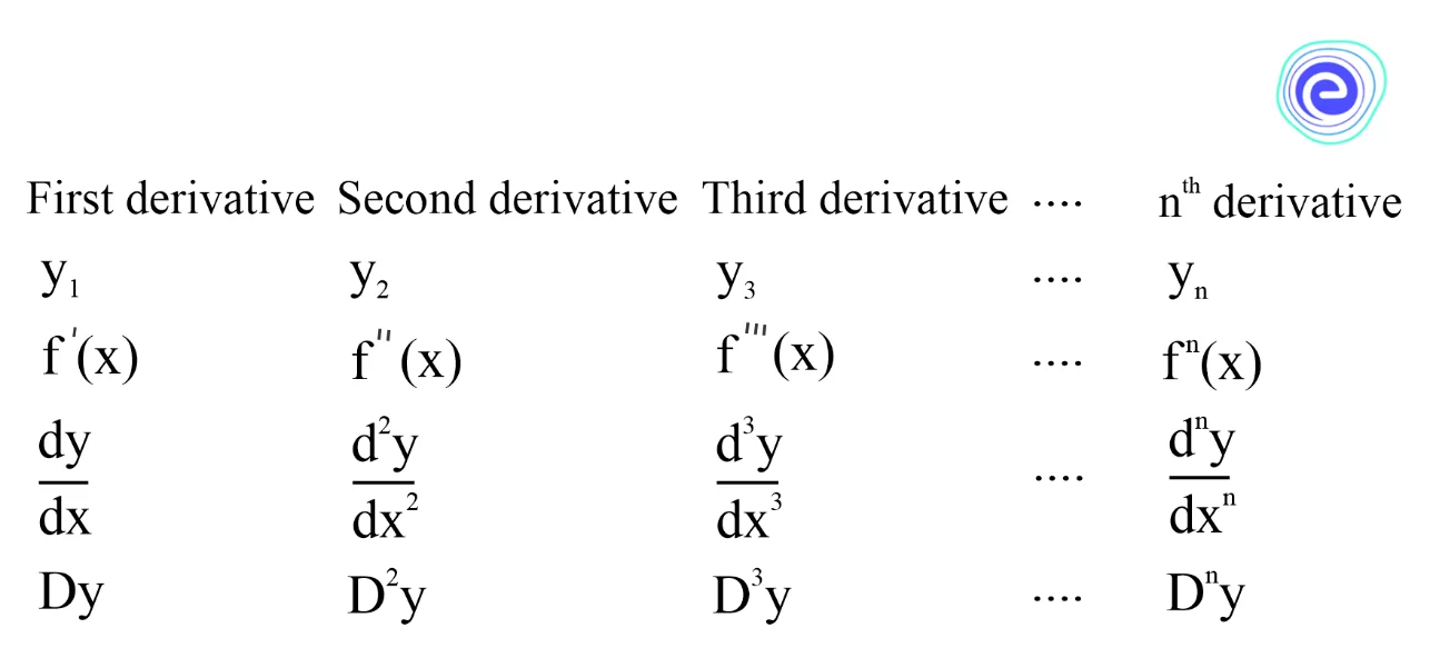
The following notations are generally used for the successive derivatives of \(y\) with respect to \(x.\)

\({n^{{\text{th}}}}\) Order Derivatives

Let us find the \({n^{{\text{th}}}}\) derivatives of few functions 

(i) Let \({y} = {e^{ax}}\)

Now, differentiate with respect to \(x,\) then we get:

 \({y_1} = a{e^{ax}}\)

Similarly, \({y_2} = {a^2}{e^{ax}}\) 

And also, \({y_n} = {a^n}{e^{ax}}\)

(ii) Let \(y = {(ax + b)^m}\)

Now, differentiate with respect to \(x,\) then we get:

 \({y_1} = ma{(ax + b)^{m – 1}}\)

Similarly, \({y_2} = m(m – 1){a^2}{(ax + b)^{m – 2}}\) 

And also, \({y_n} = m(m – 1) \ldots (m – n + 1){a^n}{(ax + b)^{m – n}}\)

  \( = \frac{{m!}}{{(m – n)!}}{a^n}{(ax + b)^{m – n}}\)

(iii) Let \(y = \log (ax + b)\)

Now, differentiate with respect to \(x,\) then we get:

 \({y_1} = \frac{a}{{(ax + b)}}\)

Similarly, \({y_2} = \frac{{ – {a^2}}}{{{{(ax + b)}^2}}}\)  and \({y_3} = \frac{{2!{a^3}}}{{{{(ax + b)}^3}}}\)

And also, \({y_n} = {( – 1)^{n – 1}}\frac{{(n – 1)!{a^n}}}{{{{(ax + b)}^n}}}\)

(iv) Let \(y = \sin (ax + b)\)

Now, differentiate with respect to \(x,\) then we get:

 \({y_1} = a\cos (ax + b) = a\sin \left( {ax + b + \frac{\pi }{2}} \right)\)

Now, \({y_2} = {a^2}\cos \left( {ax + b + \frac{\pi }{2}} \right) = {a^2}\sin \left( {ax + b + \frac{{2\pi }}{2}} \right)\)

And also, \({y_n} = {a^n}\sin \left( {ax + b + \frac{{n\pi }}{2}} \right)\)

Similarly, if \(y = \cos (ax + b),\) then \({y_n} = {a^n}\cos \left( {ax + b + \frac{{n\pi }}{2}} \right)\)

The calculation of \({n^{{\text{th}}}}\) Derivatives are given below;

Function	\({n^{{\text{th}}}}\) Derivative
\(y = {e^{ax}}\)	\({y_n} = {a^n}{e^{ax}}\)
\(y = {(ax + b)^m}\)	\({y_n} = \left\{ {\begin{array}{*{20}{c}} {\frac{{m!}}{{(m – n)!}}{a^n}{{(ax + b)}^{m – n}},}&{m > 0,m > n} \\ {0,m > 0,}&{m < n} \\ {n!{a^n},}&{m = n} \\ {\frac{{{{( – 1)}^n}n!{a^n}}}{{{{(ax + b)}^{n + 1}},}}}&{m = – 1} \end{array}} \right.\)
\(y = \log (ax + b)\)	\({y_n} = {( – 1)^{n – 1}}\frac{{(n – 1)!{a^n}}}{{{{(ax + b)}^n}}}\)
\(y = \sin (ax + b)\)	\({y_n} = {a^n}\sin \left( {ax + b + \frac{{n\pi }}{2}} \right)\)
\(y = \cos (ax + b)\)	\({y_n} = {a^n}\cos \left( {ax + b + \frac{{n\pi }}{2}} \right)\)

Leibnitz Theorem

Suppose there are two functions \(u(x)\) and \(v(x),\) which have derivatives up to \(n^{th}\) order.

Let us take the derivative of the product of these two functions;

The first derivative can be written as \((uv)’ = u’v+uv’\)

Now, if we differentiate again, then we get the second derivative as \({(uv)^{\prime \prime }} = {\left[ {{{(uv)}^\prime }} \right]^\prime }\)

\( = {\left( {{u^\prime }v + u{v^\prime }} \right)^\prime }\)

\( = {\left( {{u^\prime }v} \right)^\prime } + {\left( {u{v^\prime }} \right)^\prime }\)

\( = {u^{\prime \prime }}v + {u^\prime }{v^\prime } + {u^\prime }{v^\prime } + u{v^{\prime \prime }}\)

\( = {u^{\prime \prime }}v + 2{u^\prime }{v^\prime } + u{v^{\prime \prime }}\)

Similarly, for the third derivative, we have: \((uv)^{\prime \prime \prime }=[(uv)^{\prime \prime }]^\prime\)

\( = {\left( {{u^{\prime \prime }}v + 2{u^\prime }{v^\prime } + u{v^{\prime \prime }}} \right)^\prime }\)

\( = {\left( {{u^{\prime \prime }}v} \right)^\prime } + {\left( {2{u^\prime }{v^\prime }} \right)^\prime } + {\left( {u{v^{\prime \prime }}} \right)^\prime }\)

\( = {u^{\prime \prime \prime }}v + {u^{\prime \prime }}{v^\prime } + 2{u^{\prime \prime }}{v^\prime } + 2{u^\prime }{v^{\prime \prime }} + {u^\prime }{v^{\prime \prime }} + u{v^{\prime \prime \prime }}\)

\( = {u^{\prime \prime \prime }}v + 3{u^{\prime \prime }}{v^\prime } + 3{u^\prime }{v^{\prime \prime }} + u{v^{\prime \prime \prime }}\)

By comparing the above expressions, we see that they are very similar to binomial expansion raised to the exponent. So, if we consider the terms with zero powers, such as \({u^0}\) and \({v^0}\) which correspond to the functions \(u\) and \(v\) themselves, we can generate the formula for \({n^{{\text{th}}}}\) order of the derivative product of two functions, in such a way that,

\({(uv)^n} = \sum\limits_{i = 0}^n {\left( {\begin{array}{*{20}{c}} n \\ i \end{array}} \right)} {u^{(n – i)}}{v^i}\)

where \(\left( {\begin{array}{*{20}{l}} n\\ i \end{array}} \right)\) denotes the number of \(i-\)combinations on \(n\) elements.

This formula is known as the Leibnitz Rule.

Solved Examples – Successive Differentiation

Q.1. Find \(y_2\) for the following function \(y = {e^{3x + 2}}.\)
Ans: Given that, we have \(y = {e^{3x + 2}}……\left( i \right)\)
Now, differentiate with respect to \(x,\) then we get:
\({y_1} = \frac{{dy}}{{dx}} = {e^{3x + 2}} \cdot \frac{d}{{dx}}(3x + 2)\)
\( \Rightarrow {y_1} = {e^{3x + 2}}(3)\)
\( \Rightarrow {y_1} = 3{e^{3x + 2}} \ldots (ii)\)
Again, differentiate with respect to \(x,\) then we get:
\({y_2} = \frac{d}{{dx}}\left( {\frac{{dy}}{{dx}}} \right) = \frac{{{d^2}y}}{{d{x^2}}} = 3\left[ {{e^{3x + 2}}} \right] \cdot \frac{d}{{dx}}(3x + 2)\)
\( \Rightarrow {y_2} = 3 \cdot \left( {{e^{3x + 2}}} \right) \cdot (3)\)
\( \Rightarrow {y_2} = 9{e^{3x + 2}}\)
\(\therefore {y_2} = 9y\quad [{\rm{using}}\,\left. {(i)} \right]\)

Q.2. Find \(y_2\) for the following function \(y = \log x + {a^x}.\)
Ans: Given that, we have \(y = \log x + {a^x}\)
Now, differentiate with respect to \(x,\) then we get:
\({y_1} = \frac{{dy}}{{dx}} = \frac{1}{x} + {a^x} \cdot \log (a)\)
\( \Rightarrow {y_1} = \frac{1}{x} + {a^x}\log (a)\)
Again, differentiate with respect to \(x,\) then we get:
\({y_2} = \frac{d}{{dx}}\left( {\frac{{dy}}{{dx}}} \right) = \frac{{{d^2}y}}{{d{x^2}}} = – \frac{1}{{{x^2}}} + \log a \cdot \frac{d}{{dx}}\left( {{a^x}} \right)\)
\( \Rightarrow {y_2} = – \frac{1}{{{x^2}}} + \log a \cdot {a^x} \cdot \log a\)
\( \Rightarrow {y_2} = – \frac{1}{{{x^2}}} + {a^x}{(\log a)^2}\)

Q.3. If \(y = \log \left( {x + \sqrt {1 + {x^2}} } \right)\) then prove that \(\left( {1 + {x^2}} \right){y_{n + 2}} + (2n + 1)x{y_{n + 1}} + {n^2}{y_n} = 0\)
Ans: Given that, we have \(y = \log \left( {x + \sqrt {1 + {x^2}} } \right)\)
Now, differentiate with respect to \(x,\) then we get:
\({y_1} = \frac{1}{{x + \sqrt {1 + {x^2}} }}\left( {1 + \frac{1}{{2\sqrt {1 + {x^2}} }}2x} \right) = \frac{1}{{\sqrt {1 + {x^2}} }}\)
\( \Rightarrow \left( {1 + {x^2}} \right)y_1^2 = 1\)
Again, differentiate with respect to \(x,\) then we get:
\(\left( {1 + {x^2}} \right)2{y_1}{y_2} + 2xy_1^2 = 0\)
\( \Rightarrow \left( {1 + {x^2}} \right){y_2} + x{y_1} = 0\)
Using Leibnitz Theorem,
\(\left[ {{y_{n + 2}}\left( {1 + {x^2}} \right) + {n_{{C_1}}}{y_{n + 1}}2x + {n_{{C_2}}}{y_n}.2} \right] + \left( {{y_{n + 1}}x + {n_{{C_1}}}{y_n} \cdot 1} \right) = 0\)
\( \Rightarrow {y_{n + 2}}\left( {1 + {x^2}} \right) + {y_{n + 1}}2nx + n(n – 1){y_n} + {y_{n + 1}}x + n{y_n} = 0\)
\( \Rightarrow \left( {1 + {x^2}} \right){y_{n + 2}} + (2n + 1)x{y_{n + 1}} + {n^2}{y_n} = 0\)
Hence, proved.

Q.4. If \(y = {e^{a{{\sin }^{ – 1}}x}},\) then prove that \(\left( {1 – {x^2}} \right){y_2} – x{y_1} = {a^2}y\)
Ans: Given that, we have \(y = {e^{a{{\sin }^{ – 1}}x}}…..\left( i \right)\)
Now, differentiate with respect to \(x,\) then we get:
\({y_1} = {e^{a{{\sin }^{ – 1}}x}}\left( {a\frac{1}{{\sqrt {1 – {x^2}} }}} \right)\)
\( \Rightarrow {y_1} = \frac{{ay}}{{\sqrt {1 – {x^2}} }}\quad [{\rm{from}}\,(i)]\)
\( \Rightarrow {y_1}\sqrt {1 – {x^2}} = ay\)
Squaring on both sides, then \(y_1^2\left( {1 – {x^2}} \right) = {a^2}{y^2}\)
Again, differentiate with respect to \(x,\) then we get:
\(2{y_1}{y_2}\left( {1 – {x^2}} \right) + y_1^2( – 2x) = {a^2}\left( {2y{y_1}} \right)\)
\( \Rightarrow 2{y_1}\left[ {\left( {1 – {x^2}} \right){y_2} – x{y_1}} \right] = 2{y_1}\left( {{a^2}y} \right)\)
\( \Rightarrow \left( {1 – {x^2}} \right){y_2} – x{y_1} = {a^2}y\)
Hence, proved.

Q.5. Find the \({n^{{\rm{th}}}}\) Derivative of \(x\log x.\)
Ans: Let \(u = \log x\) and \(v = x.\) Then \({u_n} = {( – 1)^{n – 1}}\frac{{(n – 1)!}}{{{x^n}}}\) and \({u_{n – 1}} = {( – 1)^{n – 2}}\frac{{(n – 2)!}}{{{x^{n – 1}}}}\)
By using Leibnitz Theorem, we have \({(uv)_n} = {u_n}v + {n_{{C_1}}}{u_{n – 1}}{v_1} + {n_{{C_2}}}{u_{n – 2}}{v_2} + \cdots + {n_{{C_r}}}{u_{n – r}}{v_r} + \cdots + u{v_n}\)
Therefore, \({(x\log x)_n} = {( – 1)^{n – 1}}\frac{{(n – 1)!}}{{{x^n}}}x + n{( – 1)^{n – 2}}\frac{{(n – 2)!}}{{{x^{n – 1}}}} + 0\)
\( = {( – 1)^{n – 1}}\frac{{(n – 1)!}}{{{x^{n – 1}}}} + n{( – 1)^{n – 2}}\frac{{(n – 2)!}}{{{x^{n – 1}}}}\)
\( = {( – 1)^{n – 2}}\frac{{(n – 2)!}}{{{x^{n – 1}}}}[ – (n – 1) + n]\)
\( = {( – 1)^{n – 2}}\frac{{(n – 2)!}}{{{x^{n – 1}}}}\)

Summary

If \(y=f(x)\) be a function of \(x,\) then the derivative or differential coefficient of \(y\) with respect to \(x\) is denoted by \(\frac{{dy}}{{dx}}.\) If \(\frac{{dy}}{{dx}}\) can be differentiated again i.e., \(y=f(x)\) is derivable twice with respect to \(x,\) then the derivative of \(\frac{{dy}}{{dx}}\) with respect to \(x\) is denoted by \(\frac{{{d^2}y}}{{d{x^2}}}.\)

So successive differentiation is the process of finding the derivative of a function successively, and the results of such differentiation are called successive derivatives. We obtain the higher-order derivatives using the standard formula in the successive differentiations. So the higher-order derivatives are represented by \(\frac{{{d^2}y}}{{d{x^2}}},\frac{{{d^3}y}}{{d{x^3}}}\) and so on. The higher-order derivatives are of the utmost importance in scientific and engineering applications.

Frequently Asked Questions (FAQs)

Q.1. What is meant by successive differentiation?
Ans: Successive differentiation is the differentiation of a function successively to derive its higher-order derivatives with the help of the first derivative of the given function and some standard formula.

Q.2. How is successive differentiation used in real life?
Ans: The main application of successive differentiation is to find the maxima and minima of the function. Few other applications are:
1. To determine the profit and loss in business using graphs.
2. To check the temperature variation.
3. To determine the speed or distance covered, such as miles per hour, kilometre per hour etc.

Q.3. How do you find successive derivatives?
Ans: If \(y=f(x)\) be a function of \(x,\) then the derivative of \(y\) with respect to \(x\) is denoted by \(\frac{{dy}}{{dx}},\) and this is called first-order derivative. Similarly, we can find second order, third order, fourth-order, and so on with the help of first-order derivative, i.e., \(\frac{{dy}}{{dx}}\) with respect to \(x.\)

Q.4. What is the application of successive differentiation?
Ans: The successive differentiation is used in Mechanics on the graph, such as Velocity time graphs with non-linear acceleration. The slope of a velocity-time graph gives the acceleration. So, we find the acceleration by differentiating the velocity with respect to time.

Q.5. What is Leibnitz Theorem?
Ans: If \(u\) and \(v\) are functions of \(x\) such that their \({n^{{\rm{th}}}}\) derivatives exist, then the \({n^{{\rm{th}}}}\) derivative of their product is given by \({(uv)_n} = {u_n}v + {n_{{C_1}}}{u_{n – 1}}{v_1} + {n_{{C_2}}}{u_{n – 2}}{v_2} + \cdots + {n_{{C_r}}}{u_{n – r}}{v_r} + \cdots + u{v_n},\) where \({u_r}\) and \({v_r}\) represents \({r^{{\rm{th}}}}\) derivatives of \(u\) and \(v\) respectively.

We hope this detailed article on Successive Differentiation will make you familiar with the topic. If you have any inquiries, feel to post them in the comment box. Stay tuned to embibe.com for more information.